Photo by Niels Weiss on Unsplash

We introduced a large product ranking dataset in the first post in this series and established multiple zero-shot ranking baselines. In the second post, we trained ranking models using pre-trained language models and evaluated them using the NDCG ranking metric.

In this post, we dive deep into a popular method for learning to rank; gradient-boosting decision trees (GBDT). Vespa has native support for evaluating GBDT models and imports models trained with popular GBDT frameworks such as XGBoost and LightGBM.

Ranking Models

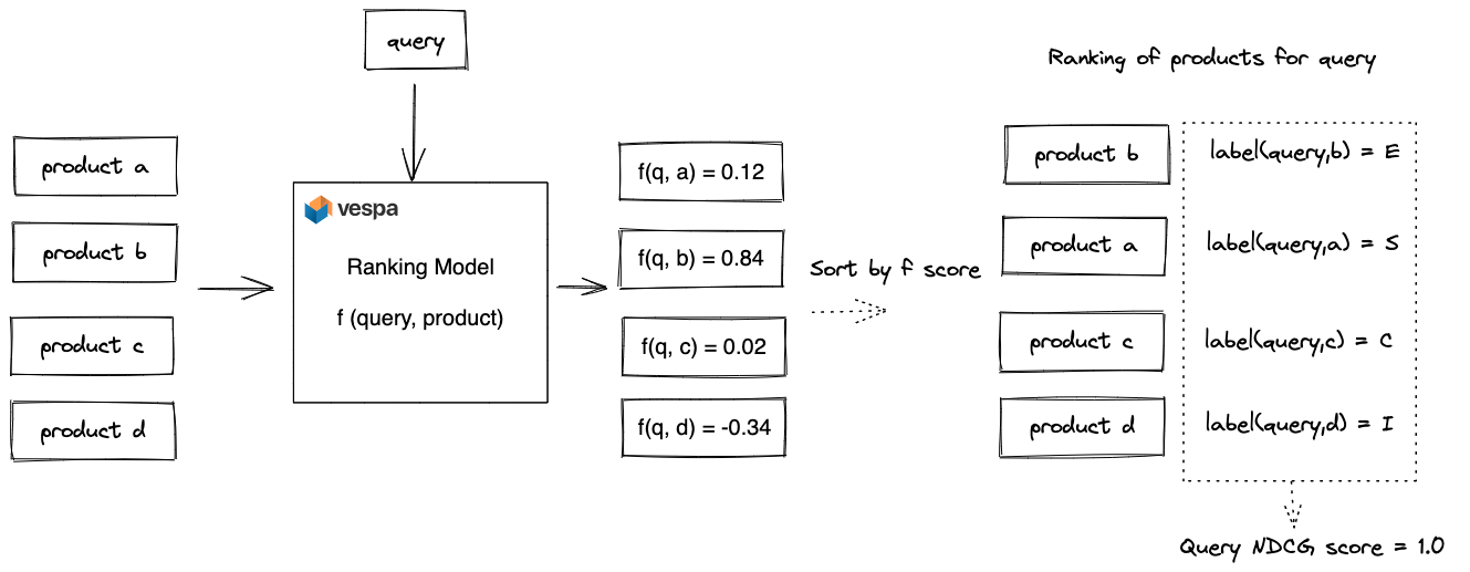
Our objective is to train a ranking model f(query, product) that takes a query and product pair as input and which outputs a relevance score. We aim to optimize the NDCG metric after sorting the products by this score. There are many ways to train a ranking model f(query, product), and in this post, we introduce and evaluate tree-based models. Tree-based GBDT models, implemented by popular frameworks like XgBoost and LightGBM, excel on tabular (structured) features and handle feature mixes and feature value ranges without any ceremony.

In our series, we only aim to optimize relevance (NDCG); still, E-commerce ranking is a multi-objective optimization problem where shops want to maximize relevance and revenue. GBDT models are famous for multi-objective ranking optimization as they handle a mix of features, combining normalized features (e.g., vector similarity), unnormalized unbound features (e.g., BM25), and “business” features such as product sales margin. GBDT is also an excellent way to explore semantic search signals and integrate them into an existing product ranking function without wasting years of ranking model development.

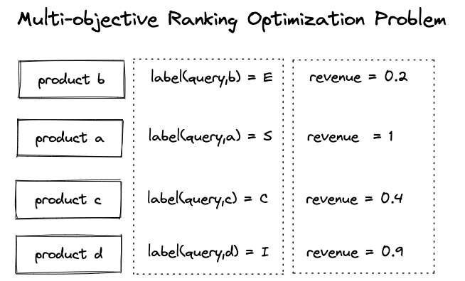
The above figure illustrates a multi-objective ranking optimization problem where we want to maximize relevance and revenue. One way to approach this problem is to train the model with a modified label, an aggregated weighted combination of the two conflicting optimization objectives.

For organizations, prediction explainability is essential when applying Machine Learning (ML) to ranking problems, and GBDT predictions are more straightforward to interpret than neural predictions. Finally, GBDT is a relatively simple algorithm, meaning we can train on more data than deep neural networks (for the same compute budget). For example, training on our product ranking dataset takes a few seconds on a laptop with CPU-only, while our neural methods from the second post took hours with GPU acceleration.

Model Features

Tree-based learning methods require tabular (structured) features. Therefore, we convert the unstructured text ranking dataset to a tabular dataset using simple feature engineering, where Vespa calculates all tabular features.

Broadly we have four classes of features used for ranking problems. Examples in this section do not necessarily map to the Amazon product ranking dataset used in this blog post series.

Contextual query features

These are features that do not depend on the document. For example, it could be the user’s age, the time of the day, or a list of previously visited products — generally, query time contextual features and the user’s query terms. Query classification techniques using language models also fall under this feature category, for example, using Vespa’s support for stateless model inference.

Document features

These features are independent of the query. In E-commerce, for example, this might be the product’s popularity, price, sale margin, or user review rating score(s).

Online match features (query * document)

An example of this could be text matching features, such as bm25(title), tensor computation like a sparse dot product between the user profile interests and product category, or semantic vector similarity, as demonstrated in the previous post in this series. See also tensor computation examples.

Aggregate features

These features aggregate across documents or queries. The computing of aggregated features is usually performed outside of Vespa, using near real-time stream processing. The output of these steam processing jobs are usually tensors which are stored and updated at scale with Vespa. Aggregate features can help cold-start problems when indexing a new document that lacks document features such as sales rank or popularity. For example, having a “category” popularity score could help rank new products added to the catalog. For example, the Yahoo homepage recommendation system uses topical click-through rate (CTR) using Vespa global tensors.

Representing features in Vespa

Vespa’s ranking framework has rich built-in features. Still, developers can easily express domain-specific features by combining Vespa’s ranking expression language with its built-in features.

Many ranking architectures in the wild use external feature stores. In these serving architectures, a middle-tier component retrieves a small pool of documents from an indexing service, for example, Elasticsearch. After retrieving documents, the middle-tier fetches features from the feature store and inputs these to the model.

Vespa allows representing a richer set of features than other traditional indexing services built on Apache Lucene. Furthermore, since Vespa stores tensor features in memory and memory bandwidth are much higher than network bandwidth, one can rank a much larger candidate pool with Vespa than with external feature stores.

Vespa attributes and tensors support in-place partial updates, and developers can update a document and aggregated features with high throughput (up to 75K partial updates/s per float field per node with low CPU resource consumption). Genuine partial update support is a feature that differentiates Vespa compared to search engines built on Apache Lucene, where partial updates trigger a full re-indexing of the entire document (get-apply-write pattern).

Gathering features from Vespa

In previous posts, we introduced Vespa rank-features and rank expressions. We can define custom features and feature computations using the Vespa rank expressions language with function support.

rank-profile features inherits default {
        inputs {
            query(query_tokens) tensor<float>(d0[32])
            query(q_title) tensor<float>(d0[384])
        } 
       
        function bi_encoder() {
            expression: closeness(field, title_embedding)
        }

        function max_title_significance() {
            expression: foreach(terms, N, term(N).significance, ">0.5", max)
        }

        function mean_title_significance() {
            expression: foreach(terms, N, term(N).significance, ">0.5", average)
        }

        first-phase {
            expression: random
        }

        match-features {
            queryTermCount
            max_title_significance
            mean_title_significance
            cross_encoder()
            bi_encoder()
            bi_encoder_description()
            bm25(title)
            bm25(description)
            fieldMatch(title)
            fieldMatch(title).proximity
        }
    }

The above features rank-profile defines a set of custom features using function with rank expressions. The match-features block defines the set of features that are returned with each ranked document. See full schema on GitHub.

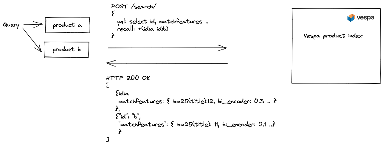
For explicitly labeled examples like in our dataset, we can ask Vespa to compute and return the feature scores using a combination of the Vespa recall parameter and match-features or summary-features. The recall query parameter allows developers to request Vespa to calculate features for query document pairs without impacting other features like queryTermCount or text matching features.

Query-product feature scraping illustration. We request that Vespa retrieve only the labeled products for each query in the train split. This feature scraping approach is used for explicit relevance judgment labels.

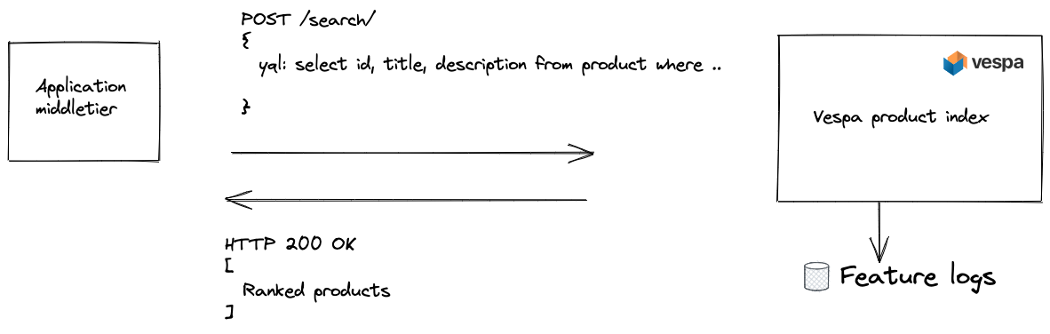
The above figure illustrates feature logging in production, and this process can be used to gather implicit relevance feedback using clicks and skips.

Feature logging infrastructure is fundamental for scaling machine learning (ML) applications beyond expensive labeled data. With Vespa, developers can compute and log new features that the current production model does not use. Vespa can log the query and the list of ranked documents with the calculated features. Note: Using click models to generate unbiased pseudo-relevance labels for model training is out of the scope of this blog post.

Generally, one wants to train on the features as scraped or logged. Computing features outside of Vespa for training might cause feature drift between training and inference in Vespa, where the offline feature computations differ from the Vespa implementation.

For our GBDT model training, we use built-in Vespa text-matching features for our product ranking datasets, such as bm25(field), nativeRank, and fieldMatch. We also include a few handcrafted function features and the neural scores from the neural bi-encoder and cross-encoder introduced in the previous post. The scrape routine fetches the computed feature values from a running Vespa instance and merges the features into a pandas DataFrame, along with the labels and query ids.

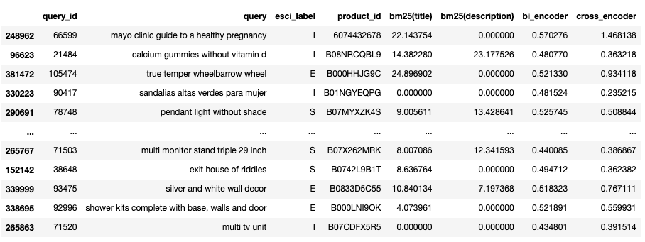
The above figure displays a random sample of tabular feature data. The DataFrame column names map 1:1 to Vespa feature names, native built-in features, or our user-defined functions, for example, bi_encoder and cross_encoder.

Gradient Boosting Decision Trees (GBDT)

This blog post won’t dive deep into how the gradient boosting algorithm works or ranking loss calculations. Instead, for our purposes, on a very high level, it suffices to say that each training iteration builds a decision tree, and each new decision tree tries to correct the errors from the previously generated decision trees.

The final model after k training iterations has k decision trees, and the model inference is performed by traversing the decision trees and summing scores in the leaf nodes of the decision trees. GBDT supports different learning objectives and loss functions:

• Classification with pointwise loss
• Regression with pointwise loss
• Ranking with listwise or pairwise ranking loss

There are two popular implementations of the GBDT algorithm; XGboost, and LightGBM; Vespa supports importing models from both frameworks. Vespa does not use the framework inference implementation but converts the models into Vespa’s ranking framework for accelerated GBDT inference. At Yahoo, Vespa has been used for ranking with GBDT models at scale long before the XGBoost and LightGBM implementations. Since the different framework models are imported into the same unified framework in Vespa, combining them into an ensemble of models from both frameworks is easy.

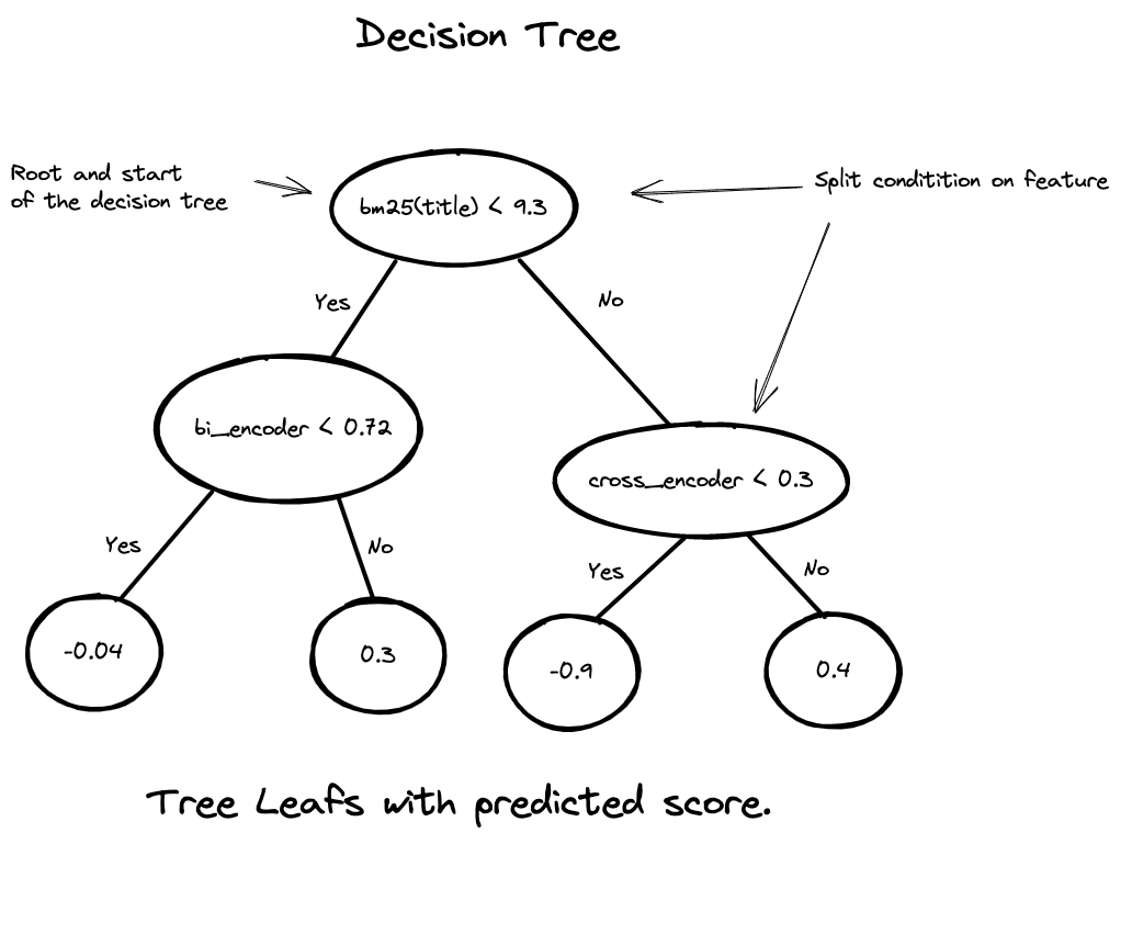
The above figure shows a single decision tree from a forest of decision trees. Each gradient-boosting learning iteration generates a new decision tree, and the final model is a forest of decision trees.

The decision tree in the illustration is two levels deep and has four leaf nodes. This simplified decision tree can only output four different scores (0.04, 0.3, -0.9, or 0.4). Each non-leaf node has a decision (split condition) that compares a feature with a numeric value. The tree traversal starts from the tree’s root, and the path determines the leaf score. The final score is the sum of all the trees in the forest.

Training GBDT models

Once we have scraped the Vespa computed features for our product ranking train data, we can start to train models. Unfortunately, it’s easy to overfit the training data with GBDT, and hyperparameters impact generalization on unseen data (test data). The previous post explained how to split the training data into a new train and dev split. Now we can use that dev split as the validation dataset used during (GBDT) training to check generalization and tune hyperparameters. The training job terminates when observed dev accuracy (NDCG) stops improving. Early termination avoids overfitting on the train set and saves resources during training and inference.

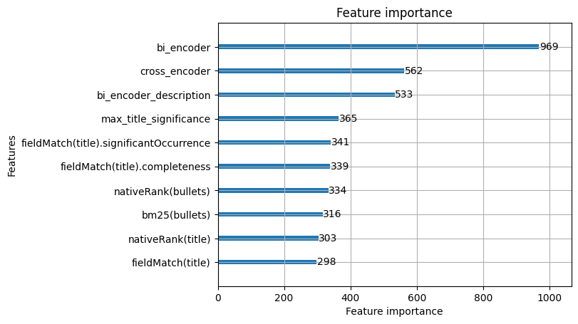
The GBDT feature importance plot enables feature ablation studies where we can remove low-importance features and re-train the model to observe the NDCG impact on the dev set. Feature importance plots allow us to reduce computational complexity and deployment costs by removing features. We make these reductions to meet a specific latency service level agreement (SLA).

In the feature importance illustration above, we have trained a model using only five simple features that are computationally simple.

GBDT models and Vespa serving performance

Training an ML model is only worthwhile if we can deploy it to production. The total computational complexity of evaluating a GBDT model for ranking in Vespa depends mainly on three factors.

The number of documents exposed to the GBDT model

The number of documents exposed to the model is the most significant parameter. Computational cost is linear with the number of documents ranked using the model. Vespa allows multiple ranking phases to apply the most computationally complex model to the top-scoring documents from the previous ranking phase. Search ranking and model inference with GBDT are highly parallelizable. Vespa’s ability to use multiple threads per query reduces serving latency.

Features and feature complexity

The number of features and the computational complexity of the features dramatically impact performance. For example, calculating a matching feature such as bm25(title) is low complexity compared to fieldMatch(title), which again is relatively low compared to inference with the previous post’s cross-encoder.

The benefit Vespa delivers is that it allows developers to understand relative feature complexity using rank tracing. The trace below shows the relative feature complexity.

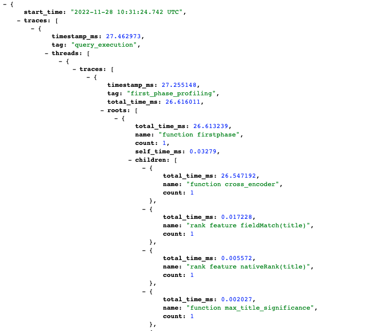
The above trace snippet is from running a query with trace.level=2 and trace.profileDepth=2. Here the total time is dominated by the expensive cross-encoder function, which is 1500 times more expensive than the second most costly feature, fieldMatch.

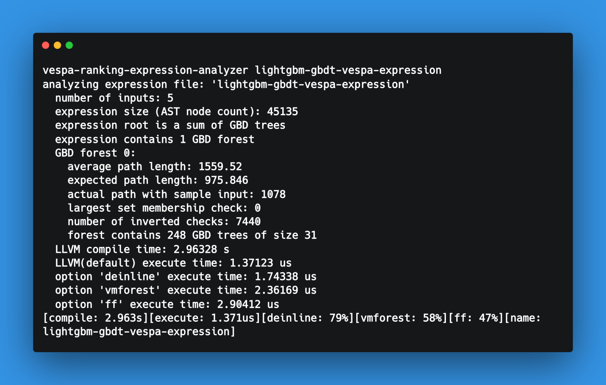
The number of trees and tree depth

The number of trees in the GBDT model impacts performance. Still, the number of trees is negligible compared to feature complexity times the number of documents ranked. Furthermore, Vespa uses LLVM to compile these ranking expressions into a program for accelerated inference. So, inference with a forest of 300-500 trees typically takes 1-3 microseconds single-threaded, and with 1000 documents, that roughly translates to 1-3 milliseconds single-threaded. Of course, we can also always parallelize the inference using more threads per query or content nodes.

Ranking Evaluation

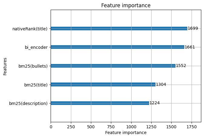
In our experiments with the product ranking dataset, we train four GBDT models using two feature sets; simple and full. The simple set uses five features with low computational complexity. The full is a more extensive feature set, including the bi-encoder and cross-encoder neural features from the previous post.

The simple feature set

• bm25(title)
• bm25(description)
• bm25(bullets)
• nativeRank(title)
• bi_encoder - The vector similarity using the trained bi-encoder model from the previous post.

The full feature set

The full feature set consist of 44 features, including the features from the simple set. See the complete feature definitions on GitHub.

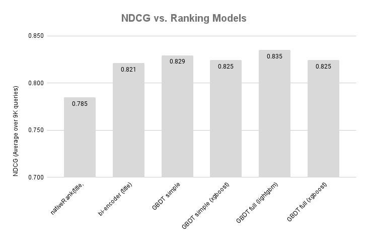
The above shows the NDCG scores for our GBDT-based models (Using the test query split). In addition, we include the best baseline zero-shot model using Vespa’s nativeRank. The resulting overall GBDT improvements over the bi-encoder are insignificant. However, we must remember that the neural methods shines with unstructured text data, and we lose information by converting the text data to tabular features.

The dataset doesn’t have features other than text. Given these parameters, models trained with XGBoost were slightly behind those trained with LightGBM. We didn’t perform any hyperparameter sweeps so the difference might be in different parameters. The model training with LightGBM is faster than XGBoost.

Another important observation is that more features may bring minor improvement. As discussed in previous sections, the number of features and their complexity-used impacts serving-related costs. Conversely, we save serving-related costs if we achieve the same accuracy (NDCG) with fewer features.

Summary

This blog post introduced GBDT methods for learning to rank, how to train the models using XGBoost and LightGBM, and how to represent the models in Vespa. We also dived into how to define and compute features with Vespa.

We have open-sourced this work as a Vespa sample app. You can reproduce the training routines using the following notebooks:

• LightGBM
• XGBoost

The notebooks are self-contained. Maybe you can tune hyperparameters to see if you can improve the NDCG score on the dev query split? Our evaluation of the test query set is end-to-end represented in Vespa.

Next Blog

In the next post in this series, scheduled for January 2023, we will deep-dive into how to perform retrieval over the product dataset discussed in this blog post series. End-to-end retrieval is a much more challenging problem than (re)-ranking. We will again produce zero-shot baselines, but now, we will remove the recall parameter and retrieve and rank over all 1.2M products. Changing the ranking problem to an end-to-end retrieval problem will introduce new challenges as we will surface products that miss relevance judgments.

We will also demonstrate how to use the train judgments to override the ranking for the queries in the train set. We (will) use our best ranking models for previously unseen queries, and we can exploit the labeled data for queries we have seen in the train set. This method can achieve 100% fit on the train queries (NDCG 1.0) while still generalizing to new, previously unseen queries (test).