Photo by Pawel Czerwinski on Unsplash

Over a few busy years, we have witnessed a neural ranking paradigm shift, where pre-trained language models, such as BERT, have revolutionized text ranking in data-rich settings with lots of labeled data. Feeding the data hungry neural networks lots of labeled relevance judgments has proved more effective than statistical (tabular) text ranking feature-based methods.

However, historically, tree-based machine learning models such as Gradient Boosting (GB) with lambdarank loss have prevailed as state-of-the-art for product search ranking. In this blog post series, we look at improving product search using learning to rank techniques, with demonstrable results on the largest publicly available product ranking dataset. We will train and measure their effectiveness on a large dataset, but without getting into the details of complex loss functions.

In this first post, we introduce a product ranking dataset and establish multiple ranking baselines that do not use the labeled relevance judgments in the dataset. These ranking models are applied in a zero-shot setting, meaning they have not been trained using domain-specific relevancy labels. The methods include traditional lexical ranking like BM25 and other Vespa native text ranking features, semantic off-the-shelf vector search models, and hybrid combinations of sparse and dense methods. All of the ranking methods are represented end-to-end in Vespa.

Dataset

In this series, we use a large shopping queries dataset released by Amazon:

We introduce the “Shopping Queries Data Set”, a large dataset of complex search queries released to foster research in semantic matching of queries and products. For each query, the dataset provides a list of up to 40 potentially relevant results, together with ESCI relevance judgments (Exact, Substitute, Complement, Irrelevant) indicating the relevance of the product to the query. Each query-product pair is accompanied by additional information. The dataset is multilingual, containing queries in English, Japanese, and Spanish.

The dataset consists of a large number of questions, and where each query has, on average, 20 graded query-item relevance judgments:

• Exact (E): the item is relevant to the query and satisfies all the query specifications (e.g., water bottle matching all attributes of a query “plastic water bottle 24oz”, such as material and size)

• Substitute (S): the item is somewhat relevant: it fails to fulfill some aspects of the query, but the item can be used as a functional substitute (e.g., fleece for a “sweater” query)

• Complement (C): the item does not fulfill the query but could be used in combination with an exact item (e.g., track pants for “running shoe” query)

• Irrelevant (I): the item is irrelevant, or it fails to fulfill a central aspect of the query (e.g., socks for a “pant” query)

As with most ranking datasets, the dataset is split into a train and test part, and models can be trained using the train split and evaluated on the test split. In our work, we focus on the English queries in both splits.

English Train Split

The train split contains 20,888 queries with 419,653 query-item judgments. This split can be used to train models, using learning to rank techniques. The train set will be the focus of upcoming blog posts.

English Test Split

In this blog post we focus on the test split, and it contains 8,956 queries with 181,701 query-item judgments.

The judgment label distribution is as follows:

• Exact (Relevant) 79,708 (44%)
• Substitute (Somewhat Relevant) 8,099 (4%)
• Complement 63,563 (35%)
• Irrelevant 30,331 (17%)

Both splits have about 20 product judgments per query. As we can see from the label distribution, the dataset has many Exact (relevant) judgments, especially compared to Substitutes (somewhat relevant) and Irrelevant. On average, there are about 9 relevant products for every query in the test split.

This product relevance dataset is the largest available product relevance dataset and allows us to compare the effectiveness of multiple ranking models using graded relevance judgments. A large dataset allows us to report information retrieval ranking metrics and not anecdotical LGTM@10 (Looks Good To Me) metrics.

We can evaluate ranking models used in a zero-shot setting without using the in-domain relevance labels and models trained using learning to rank techniques, exploiting the relevance labels in the train split.

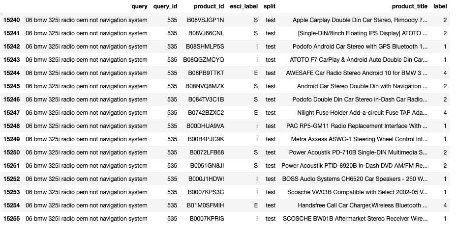
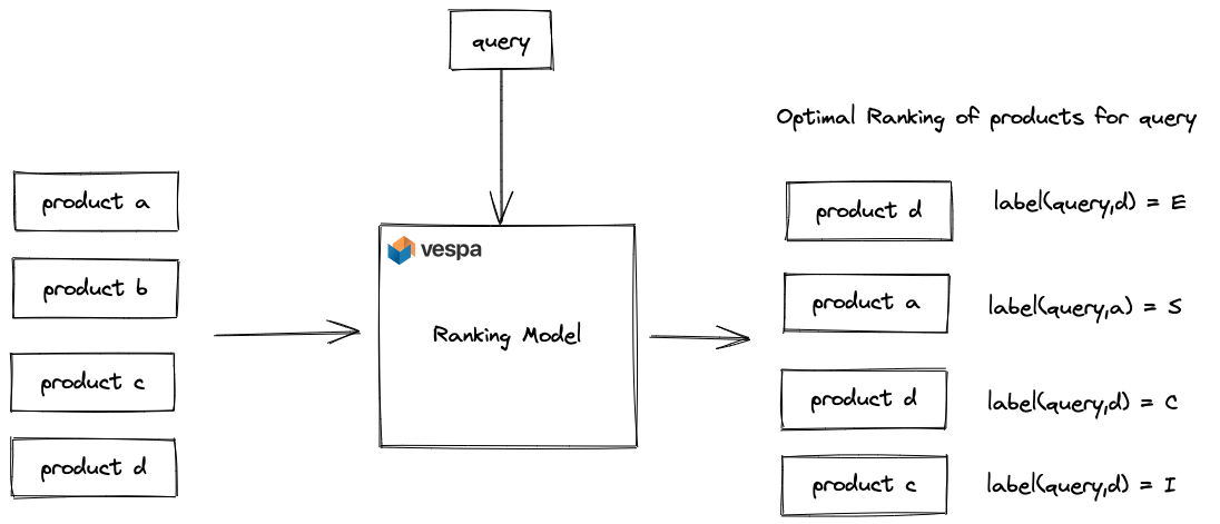
The above image shows query #535 in the test split with a total of 16 product judgements. The task is to optimize the ordering (ranking) so that products labeled as exact are ordered before supplements and supplements before irrelevant.

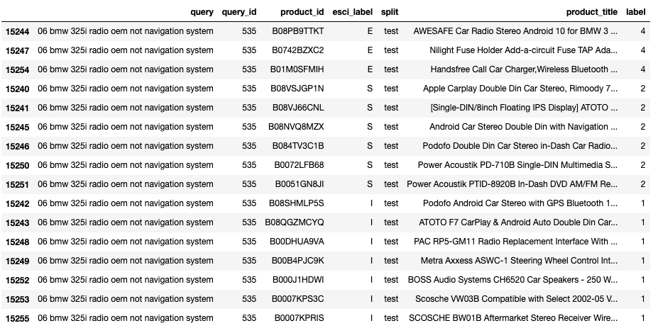The above image shows perfect ranking of products for query #535. Note that we have converted the textual labels (esci_label) to numeric labels using E=4, S=3, C=2, I=1. If our ranking function is able to produce this ordering, we would get a perfect score for this query.

Indexing the dataset with Vespa

We use the following Vespa document schema, which allows us to index all the products associated with English queries across both splits. We use a utility script that converts the parquet product data file to a Vespa JSON formatted feed file. In total we index about 1.2M products in Vespa.

schema product {

    document product {

        field id type string {
            indexing: summary | index 
            rank:filter
            match:word
        }

        field title type string {
            indexing: summary | index
            index: enable-bm25
            match:text
            weight:300
            bolding:on
        }

        field description type string {
            indexing: summary | index
            index: enable-bm25
            match:text
            weight: 200
        }

        field bullets type string {
            indexing: summary | index
            index: enable-bm25
            match:text
            weight: 200
        }

        field brand type string {
            indexing: summary | index | attribute
            match:text
            weight:100
        }

        field color type string {
            indexing: summary | index | attribute
            match:text
            weight:100
        }

    }

    field title_tokens type tensor<float>(d0[32]) {
        indexing: input title | embed tokenizer | attribute
    }

    field description_tokens type tensor<float>(d0[128]) {
        indexing: input description | embed tokenizer | attribute
    }

    field embedding type tensor<float>(d0[384]) {
        indexing {
            input title . input description | embed transformer | attribute | summary | index
        }
        attribute {
            distance-metric: angular 
        }
    }
    fieldset default {
        fields: title, description, bullets, brand  
    }
}

The product data contains title, description, brand, color and bullets. We use Vespa’s support for encoding text into vector embeddings, in this case we use the title and description as input. See text embedding made simple for details on how to embed text embedding models in Vespa.

Evaluation

The official dataset evaluation metric is NDCG (Normalized Discounted Cumulative Gain), a precision-oriented metric commonly used for ranking datasets with graded relevance judgments. An important observation is that the task only considers ranking of the products that have judgment labels. In other words, we assume that a magic retriever has retrieved all relevant documents (plus irrelevant documents), and our task is to re-rank the products so that the relevant ones are pushed to the top of the ranked list of products. This is a simpler task than implementing end-to-end retrieval and ranking over the 1.2M products.

Many deployed search systems need to hedge the deployment cost and deploy multi-phased retrieval and ranking pipelines to reduce computational complexity. In a retrieval and ranking funnel, one or many diverse retrievers use a cost-efficient retrieval ranking phase, and subsequent ranking phases re-rank the documents, focusing on precision. In a later post in this series, we look at how to train a retriever function using learning to retrieve and how to represent retrieval and ranking phases in Vespa.

Baseline zero-shot ranking models

We propose and evaluate seven different baseline ranking models, all represented end-to-end in Vespa using Vespa’s ranking framework.

Random

Obviously not the greatest baseline, but allows us to compare other baselines with random ranking. We use Vespa’s random rank-feature.

A pseudorandom number in the range [0,1] which is drawn once per document during rank evaluation.

rank-profile random inherits default {
    first-phase {
        expression: random 
    }
}

BM25 - lexical ranking

BM25 is a tried and true zero-shot text ranking model. BM25 only has two parameters and is the ranking function many turn to when there are no explicit relevancy labels or implicit click feedback to train ranking models. The BM25 scoring function can also be accelerated for efficient retrieval using dynamic pruning algorithms like WAND.

rank-profile bm25 inherits default {
    first-phase {
        expression: bm25(title) + bm25(description) 
    }
}

Note that we only use the title and description. All our lexical baselines uses only these two fields.

Vespa nativeRank - lexical ranking

Vespa’s nativeRank is a lexical ranking function and the default text ranking function in Vespa. It has similar characteristics as BM25 but also considers the proximity between matched terms in the document. Unlike BM25, which has an unbound score range, Vespa’s nativeRank is normalized to a score in the range [0,1].

rank-profile nativeRank inherits default {
    first-phase {
        expression: nativeRank(title) + nativeRank(description) 
    }
}

Vespa fieldMatch - lexical ranking

Vespa fieldMatch is another lexical ranking function that is more sophisticated than Vespa nativeRank but also computationally expensive and unsuitable as a retrieval function. fieldMatch(field) or fieldMatch sub-features such as fieldMatch(field).proximity is typically used as re-ranking features.

rank-profile fieldMatch inherits default {
    first-phase {
        expression: fieldMatch(title) + fieldMatch(description) 
    }
}

Vespa semantic ranking using vector similarity - dense retrieval

Using an off-the-shelf dense vector model from Huggingface, we encode documents and queries into a 384-dimensional dense vector space. We use cosine similarity between the query and the document in this shared embedding vector space as our relevancy measure. The vector embedding model, sentence-transformers/all-MiniLM-L6-v2, is trained on a large number of sentence-length texts.

Semantic similarity search over dense representations can be accelerated using Vespa‘s support for approximate nearest neighbor search, making it usable for efficient retrieval. We use Vespa’s support for embedding dense embedding models in this work. See text embeddings made simple.

rank-profile semantic inherits default {
    inputs {
        query(query_embedding) tensor<float>(d0[384])
    } 
    first-phase {
        expression: closeness(field, embedding)
    }
} 

Vespa semantic ranking using vector similarity - dense retrieval

Another model that can be used for vectorization, bert-base-uncased, 768-dimensional. This model has not been trained for semantic similarity, or semantic search. We use the pre-trained language model directly. As with the previous semantic model, we use cosine similarity between the query and the document as our relevancy measure.

rank-profile semantic inherits default {
    inputs {
        query(bert_query_embedding) tensor<float>(d0[768])
    } 
    first-phase {
        expression: closeness(field, bert_embedding)
    }
} 

Vespa hybrid - combining lexical and semantic ranking

In this baseline model, we combine the semantic similarity score of the sentence-transformers/all-MiniLM-L6-v2 model with the lexical score computed by Vespa’s nativeRank. We use a simple linear combination of the two ranking models. Since the nativeRank lexical feature is normalized in the range [0,1], combining it with semantic similarity is more straightforward as we don’t need to normalize unbound lexical scoring functions, such as BM25. We use a query(alpha) parameter to control how each method influences the overall score.

rank-profile hybrid inherits default {
    inputs {
        query(alpha): 0.5
        query(query_embedding) tensor<float>(d0[384])
    }
    first-phase {
        expression: query(alpha)*closeness(field, embedding) + (1 - query(alpha))*(nativeRank(title) + nativeRank(description))
    }
}

Zero-shot Baseline Results

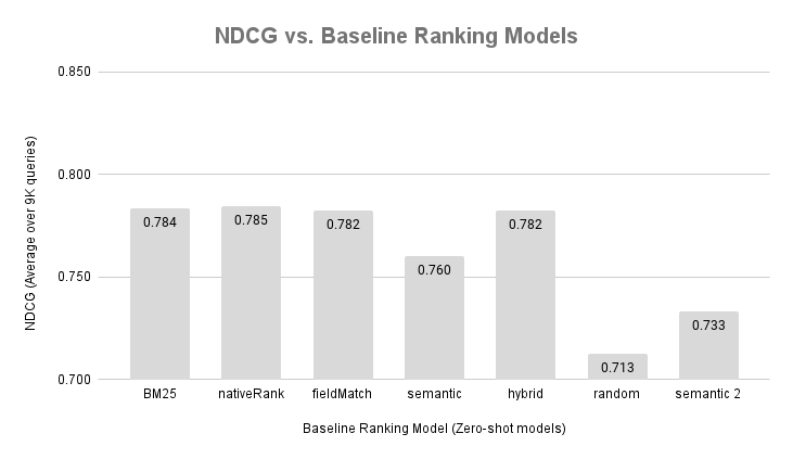
We present the results of our evaluation in the above figure. We execute each query in the English test split (8.9K queries) and ask Vespa to rank the documents that we have labels for, using the Vespa search API’s recall parameter.

Sets a recall parameter to be combined with the query. This is identical to filter, except that recall terms are not exposed to the ranking framework and thus not ranked.

We use trec_eval utility to compute NDCG, using the relevance judgments. The reported NDCG is the average NDCG calculated across all 8,956 queries in the test split. These are unique queries and we don’t know their frequency distribution on Amazon, but in a real-world evaluation we would have to take into account the query frequency as well when evaluating the model, for example using weighting so that popular (head) queries weights more than rare (tail) queries. In other words, we don’t want to introduce a ranking model that on average improves NDCG, but hurts many head queries.

Notice that the random ranking function produces a high NDCG score, this is because there are many exact (relevant) judgements per query. On average, 9 out of 20 judgments per query is exact. This demonstrates that including a random baseline has value, since it allows us to compare other models to a random baseline.

The semantic 2 is the bert-base-uncased model. A model which have not been fine-tuned for retrieval or ranking tasks, but masked-language-modeling. The bert-base-uncased NDCG score is closest to the random baseline. This demonstrates that not all vectorization models that encode text into vectors are great for ranking. In addition, the bert-base-uncased model is about 5x larger than the model used in semantic model 1, which costs both storage (dimensionality), and CPU cycles during inference.

The semantic model 1, which is the sentence-transformers/all-MiniLM-L6-v2 model, also underperforms compared to the lexical based methods. This is a known shortcoming with dense vectorization models, they might not work well in a zero-shot setting when applied on a new text domain.

In this dataset, the hybrid combination of lexical (nativeRank) and semantic did not yield any improvement over the pure lexical ranking methods. We did not tune the alpha parameters, as tuning parameters to improve accuracy on the test set is a bad machine learning practice.

Summary

In this blog post, we described a large product relevance dataset and evaluated several baseline ranking methods on this dataset, applied in a zero-shot setting.

In the next blog post in this series, we will use the labeled train split of the dataset to train multiple ranking models using various learning to rank techniques:

• A semantic similarity model using two-tower/ bi-encoder architecture. Building on a pre-tuned model, we will use the training data (query product labels) to fine-tune the model for the product ranking domain. We then embed this model into Vespa for semantic search.

• A semantic cross-encoder similarity model based on a pre-trained language model. A more computationally expensive model than bi-encoders, but generally more accurate than bi-encoders that reduces semantic similarity to a vector similarity.

• Gradient Boosting (GB) models, combining multiple ranking signals. GB models are famous for their performance on tabular data and popular in e-commerce search ranking. We include GB methods, as historically, these models have been prevalent for product search ranking, including statistical features such as sales rank or other business-logic-oriented features. We will use a combination of lexical and neural features and feed into the GB model. For run-time inference, we will be using Vespa’s support for LightGBM and XGBoost models, two popular frameworks for GBDT models.

• Ensemble ranking models. Since Vespa maps different models from different frameworks into the same ranking framework, combining multiple models into an ensemble model is straightforward.