

Photo by Patrick Hendry on Unsplash
Updated 2022-10-21: Added links and clarified some sections
In this blog series we demonstrate how to represent transformer models in a multiphase retrieval and ranking pipeline using Vespa.ai. We also evaluate these models on the largest Information Retrieval relevance dataset, namely the MS Marco Passage ranking dataset. We demonstrate how to achieve close to state of the art ranking using miniature transformer models with just 22M parameters, beating large ensemble models with billions of parameters.
Blog posts in this series:
- Post one: Introduction to neural ranking and the MS Marco passage ranking dataset
- Post two: Efficient retrievers, sparse, dense, and hybrid retrievers
- Post three: Re-ranking using multi-representation models (ColBERT)
- Post four: Re-ranking using cross-encoders
In the first post in this series we introduced using pre-trained language models for ranking and three popular methods for using them for text ranking. In the second post we studied efficient retrievers which could be used as the first phase in a multiphase retrieval and ranking pipeline. In the third post we studied the ColBERT re-ranking model.
In this fourth and last post in our blog post series on pre-trained transformer models for search, we introduce a cross-encoder model with all-to-all interaction between the query and the passage.
We deploy this model as our final ranking stage in our multiphase retrieval and ranking pipeline, furthermore, we submit the ranking results to the MS Marco Passage Ranking Leaderboard.
In addition, we benchmark the serving performance of all the retrieval and ranking methods introduced in this blog post series. Finally, we also release a vespa sample application, which lets try out these state of the art retrieval and ranking methods.
Introduction
In this blog post we study the third option for using transformer models for search and document ranking. This option is the simplest model to configure and use in Vespa but also the most computationally expensive model in our multi-phase retrieval and ranking pipeline. With the cross attention model we input both the query and the passage to the model and as we know by now, the computational complexity of the transformer is squared with regards to the input length. Doubling the sequence length increases the computational complexity by 4x.
The cross-encoder model is a transformer based model with a classification head on top of the Transformer CLS token (classification token). The model has been fine-tuned using the MS Marco passage training set and is a binary classifier which classifies if a query,document pair is relevant or not.
The cross-encoder model is also based on a 6-layer MiniLM model with only 22.7M parameters, same as the transformer models previously introduced in this blog series. As with the other two transformer models we introduced in previous posts in this series, we integrate this model in Vespa using ONNX format. The model is hosted on the Huggingface model hub.
We use a quantized version where the original float weights have been quantized to int8 representation to speed up inference on cpu.
Vespa representation of the cross-encoder model
In previous posts we have introduced the Vespa passage schema. We add a new tensor field to our schema and in this tensor field we will store the transformer token ids of the processed text. We haven’t described this in detail before, but the MiniLM model uses as input the sequence of the numeric token ids from the fixed BERT token vocabulary of about 30K unique tokens or subwords.
For example the passage:
Charles de Gaulle (CDG) Airport is close to Paris
Is tokenized to:
['charles', 'de', 'gaulle', '(', 'cd', '##g', ')', 'airport', 'is', 'close', 'to', 'paris']
The subword tokens are mapped to token ids from the fixed vocabulary, e.g ‘charles’ maps to token id 2798. The example passage text is represented as a tensor by:
[2798, 2139, 28724, 1006, 3729, 2290, 1007, 3199, 2003, 2485, 2000, 3000]
We use the native Vespa WordPiece embedder to map the text into tensor representation.
The passage document schema, including the new text_token_ids field:
search passage {
  document passage {
    field id type int {...}
    field text type string {...}
    field mini_document_embedding type tensor<float>(d0[384]){...}
    field dt type tensor<bfloat16>(dt{}, x[32]){..}
  }

  field text_token_ids type tensor<float>(d0[128])  {
    indexing: input text | embed tokenizer | attribute | summary
    attribute: paged
  }
}
We store maximum 128 tokens, denoted by d0[128]. This is an example of an indexed Vespa tensor type.
Vespa ranking with cross-encoder model
We are going to use the dense retriever model, accelerated by Vespa’s approximate nearest neighbor search to efficiently retrieve passages for re-ranking with our transformer based ranking models. The retrieved hits are re-ranked with the ColBERT model introduced in the third post, and finally the top ranking documents from the ColBERT model is re-ranked using the cross-encoder.
The retrieval and ranking pipeline have two re-ranking depth parameters.
- How many are re-ranked with ColBERT is determined by the target number of hits passed to the nearest neighbor query operator.
- The number of documents that are re-ranked using the final cross-encoder model is determined by the rank-profile rerank-count property.
See phased ranking with Vespa. Both these parameters impact end-to-end serving performance and also ranking accuracy as measured by MRR@10.
Both the nearest neighbor search target number of hits and rerank-count is per content node which is involved in the query. This is only relevant for deployments where the document corpus cannot be indexed on a single node due to either space constraints (memory, disk) or serving latency constraints.
Defining the MiniLM cross-encoder
schema passage {
  document passage {...}

  onnx-model minilmranker {
    file: files/ms-marco-MiniLM-L-6-v2-quantized.onnx
    input input_ids: input_ids
    input attention_mask: attention_mask
    input token_type_ids: token_type_ids
  }
}
In the above snippet we define the ONNX model and its inputs, each of the inputs are mapped to a function declared later in the ranking profile. Each function produces a tensor which is used as input to the model. The file points to the ONNX formatted model format, placed in in src/main/application/files/. Vespa takes care of distributing the model to the content node(s). The inputs to the model are standard transformer inputs (input_ids, attention_mask and token_type_ids).
The first part of the ranking profile where we define the 3 input functions to the BERT model looks like this:
  rank-profile dense-colbert-mini-lm {
    function input_ids() {
       expression: tokenInputIds(128, query(query_token_ids), attribute(text_token_ids))
    }
    function token_type_ids() {
      expression: tokenTypeIds(128, query(query_token_ids), attribute(text_token_ids))
    }
    function attention_mask() {
      expression: tokenAttentionMask(128, query(query_token_ids), attribute(text_token_ids))
    }
}
For example the input input_ids the function input_ids which is defined as
  function input_ids() {
       expression: tokenInputIds(128, query(query_token_ids), attribute(text_token_ids))
    }
For example, for a text query
is CDG in paris?
The query tensor representation becomes:
[2003, 3729, 2290, 1999, 3000, 1029]
The tokenInputIds ranking function will create the concatenated tensor of both query and passage including the special tokens. Using the example passage from previous section with the above query example our concatenated output with special tokens becomes:
[101, 2003, 3729, 2290, 1999, 3000, 1029, 102, 2798, 2139, 28724, 1006, 3729, 2290, 1007, 3199, 2003, 2485, 2000, 3000, 102]
Where 101 is the CLS token id and 102 is the SEP token separating the query from the passage.
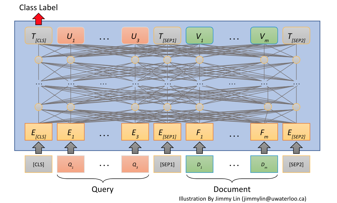
The above figure illustrates the input and output of the cross-encoder transformer model.
Notice the CLS output embedding which is fed into the classification layer which predicts the class label (Relevant = 1, irrelevant = 0).
Now as we have presented how to represent the cross-encoder model, we can present the remaining parts of our ranking profile:
rank-profile dense-colbert-mini-lm {
    ...

    function maxSimNormalized() {
      expression {
        sum(
          reduce(
            sum(
              query(qt) * attribute(dt), x
            ),
            max, dt
          ),
          qt
        )/32.0
       }
    }
    function dense() {
      expression: closeness(field, mini_document_embedding)
    }

    function crossModel() {
      expression: onnx(minilmranker){d0:0,d1:0}
    }

    first-phase {
        expression: maxSimNormalized()
    }

    second-phase {
      rerank-count: 24
      expression: 0.2*crossModel() + 1.1*maxSimNormalized() + 0.8*dense()
    }
}
The maxSimNormalized function computes the ColBERT MaxSim function which we introduced in post 3, here we also normalizes the MaxSim score by dividing the score with 32 which is the configured max ColBERT query encoder query length, and each term has maximum score of 1.
The dense() function calculates the cosine similarity as calculated by the dense retriever introduced in post 2
In the crossModel() function we calculate the score from cross-encoder introduced in this blog post:
function crossModel() {
  expression: onnx(minilmranker){d0:0,d1:0}
}
The {d0:0,d1:0} access the logit score. (d0:0 is the batch dimension, which always is of size 1, and d1:0 access the logit score, which is a proxy for the relevancy).
Ranking profile summarized
- Retrieve efficiently using the dense retriever model - This is done by the Vespa approximate nearest neighbor search query operator.
- The k passages retrieved by the nearest neighbor search is re-ranked using the ColBERT MaxSim operator. K is set by the target hits used for the nearest neighbor search.
- In the last phase, the top ranking 24 passages from the previous phase are evaluated by the cross attention model.
- The final ranking score is a linear combination of all three ranking scores. The rerank-count can also be adjusted by a query parameter
Observe that reusing scores from the previous ranking phases does not impact serving performance, as they are only evaluated once (per hit) and cached.
The linear weights of the three different transformer scores was obtained by a simple grid search observing the ranking accuracy on the dev query split when changing parameters.
MS Marco Passage Ranking Submission
We submitted a run for the MS Massage Ranking where we used targetHits 1K for the approximate nearest neighbor search, so that 1K passages are re-ranking using the ColBERT model and finally 96 passages are re-ranked with the cross-encoder model.
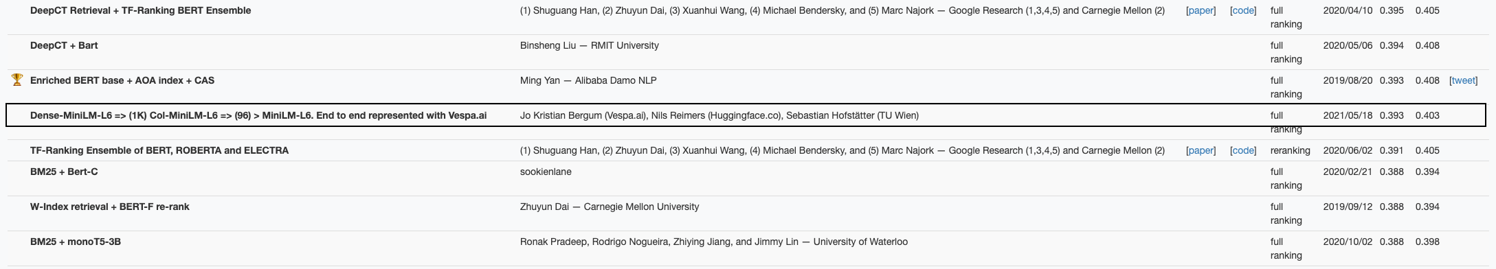
Our multi-phase retrieval and ranking pipeline with 3 miniature models performed pretty well, even beating large models using T5 with 3B parameters. See MS Marco Passage Ranking Leaderboard.
| Model | Eval | Dev |
|---|---|---|
| BM25 (Official baseline) | 0.165 | 0.167 |
| BM25 (Lucene8, tuned) | 0.190 | 0.187 |
| Vespa dense + ColBERT + cross-attention | 0.393 | 0.403 |
Multi-threaded retrieval and ranking
Vespa has the ability to use multiple threads per search query. This ability can reduce search latency as the document retrieval and ranking for a single query can be partitioned, so that each thread works on a subset of the searchable documents in an index. The number of threads to use is controlled on a per rank profile basis, but can only use less than the global setting controlled in the application services.xml.
To find optimal settings, we recommend benchmarking starting with one thread per search and increasing until latency does not improve significantly. See Vespa Scaling Guide for details.
Serving performance versus ranking accuracy
In this section we perform benchmarking where we deploy the system on a Vespa cloud instance using 2 x Xeon Gold 6263CY 2.60GHz (HT enabled, 48 cores, 96 threads) with 256GB memory.
We use a single content node indexing the 9M passages. All query encodings with the MiniLM based query encoders, retrieval and re-ranking is performed on this content node. We also use 2 stateless container nodes with 16 v-cpu each to make sure that we are benchmarking the content node performance. See Vespa overview on stateless container nodes versus content nodes.
Running everything of importance on the same node enables us to quantitatively compare the performance of the methods we have introduced in this blog post series. We benchmark throughput per retrieval and ranking model until we reach about 70% cpu utilization, and compare obtained throughput and latency. We also include tail latency (99.9 percentile) in the reported result.
We use the vespa-fbench benchmarking utility to load the cluster (by increasing the number of clients to reach about 70% cpu util). We use the queries from the development set which consist of 6980 unique queries, the same query might be repeated multiple times, but there is no result caching enabled.
A real world production setup would benefit from caching the result of the two query models, and one would expect a high cache hit ratio for real-world natural language queries.
For the sparse retrieval, using the Vespa WAND query operator, which might touch the disk, we pre-warm the index by running through the dev queries once. In reality, sparse retrieval with WAND will have worse performance than reported here, when running with continuous indexing due to IO buffer cache misses.
Benchmarking Results
We summarize the benchmark result in the table below. These are end-to-end benchmarks using the Vespa http serving api, also including query encoding(s).
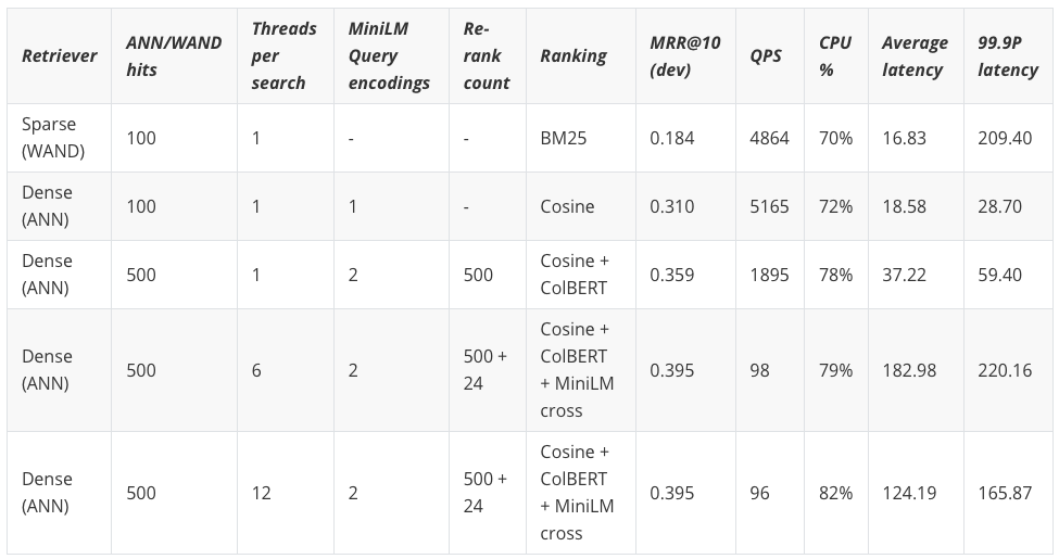
The Dense(ANN) retrieval method, using approximate nearest neighbor search, is both evaluated as a single stage retriever without re-ranking and with ColBERT re-ranking.
The final experiment uses both ColBERT and the Cross-Encoder. The dense single stage retriever using approximate nearest neighbor search, has on average slightly worse latency than sparse (wand), but wins in throughput and also less latency variation (e.g 99.9P).
It is known that sparse retrieval using WAND will have different latency or cost, depending on the number of query terms in the query. Dense retrieval on the other hand maps the query terms into a dense representation, and is not sensitive to the number of query terms.
For dense retrieval using ANN there is only one query encoding through the MiniLM model, while every ranking model which uses ColBERT also needs to encode the query through the ColBERT query encoder model. The encoding steps are performed in parallel to avoid sequential latency.
Notice that the last re-ranking phase using the cross-encoder drives the overall cost up significantly. From 1895 QPS @ 0.359 MRR@10 to less than 100 QPS @ 0.395 MRR@10. In other words, to improve ranking accuracy by 10% from 0.359 to 0.395 the cost increases by close to 18x. This increase in cost, can be worth it in many cases, as 10% is a significant improvement.
Summary
In this blog post we have demonstrated how to represent a cross-encoder model as final re-ranking step on top of the previous retrieval and ranking methods introduced in previous blog posts.
- Representing the cross-encoder model in Vespa ranking framework.
- Multi-phase retrieval and ranking using three phases (dense retrieval, ColBERT re-ranking and finally cross-encoder re-ranking).
- Documented the performance versus accuracy trade-offs for production deployments.
- Dense retrieval accelerated by nearest neighbor search versus sparse retrieval accelerated by the dynamic pruning WAND algorithm.
Now, you can go check out our vespa sample application which lets you try out these state-of-the-art retrieval and ranking methods.