Photo by Carl Campbell on Unsplash

In the first post, we introduced a large product ranking dataset and established multiple zero-shot ranking baselines that did not use the labeled relevance judgments in the dataset. In this post, we start exploiting the labeled relevance judgments to train deep neural ranking models. We evaluate these models on the test set to see if we can increase the NDCG ranking metric.

Dataset Splits

The English train split contains 20,888 queries with 419,653 query-item judgments. To avoid training and tuning models based on observed test set accuracy, we split the official train set into two new splits; train and dev. In practice, we pick, at random, 20% of the queries from the train as our dev split and retain the remaining 80% as train queries.

Since we plan to train multiple models, we can use the performance on the dev set when training ensemble models and then hide the dev set during the training.

Train Original: 20,888 queries with 419,653 judgments

• Our Train 16,711 queries with 335,674 assessments
• Our Dev 4,177 queries with 83,979 assessments

We do this dataset split once, so all our models are trained with the same train and dev split.

Ranking Models

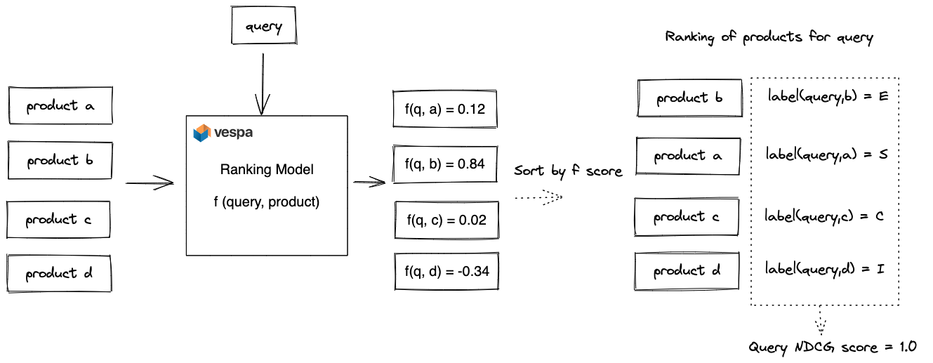
Our objective is to train a ranking model f(query,product) that takes a query and product pair and outputs a relevance score. We aim to optimize the NDCG ranking metric after sorting the products for a query by this score.

The ranking process is illustrated for a single query in the above figure. We are asked to rank four products for a query with model f. The model scores each pair and emits a relevance score. After sorting the products by this score, we obtain the ranking of the products for the query. Once we have the ranked list, we can calculate the NDCG metric using the labeled query and product data. The overall effectiveness of the ranking model is given by computing the average NDCG ranking score for all queries in the test dataset.

There are many ways to train a ranking model f(query, product), and in this post, we introduce and evaluate two neural ranking methods based on pre-trained language models.

Neural Cross-Encoder using pre-trained language models

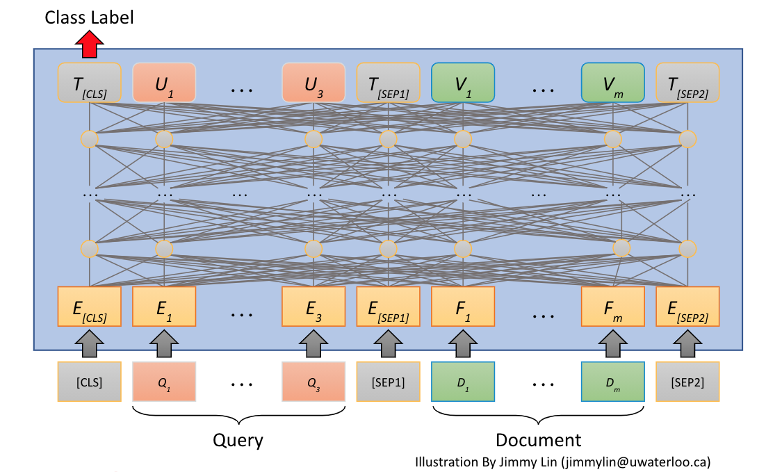
One classic way to use Transformers for ranking is cross-encoding, where both the query and the document are fed into the Transformer model simultaneously.

The simultaneous input of the query and document makes cross-encoders unsuitable for cost-efficient retrieval. In this work, we are relatively lucky because we already have a magic retriever, and our task is to re-rank a small set (average 20) of products per query.

One approach for training cross-encoders for text ranking is to convert the ranking problem to a regression or classification problem. Then, one can train the model by minimizing the error (loss) between the model’s predicted and true label. A popular loss function for regression and classification problems is MSE (Mean Squared Error) loss. MSE loss is a pointwise loss function, operating on a single (query, document) point when calculating the error between the actual and predicted label. In other words, the pointwise loss function does not consider the ranking order of multiple (query, document) points for the same query. In the next blog post in this series we will look at listwise loss functions.

With graded relevance labels, we can choose between converting the ranking problem to a regression (graded relevance) or binary classification (relevant/irrelevant) problem. With binary classification, we need to set a threshold on the graded relevance labels. For example, let Exact and Complement map to the value 1 (relevant) and the remaining labels as 0 (irrelevant). Alternatively, we can use a map from the relevancy label to a numeric label representation.

Exact => 1.0, Substitute => 0.1, Complement => 0.01, Irrelevant => 0

With this label mapping heuristic, we “tell” the model that Exact should be 10x as important as Substitute and so forth. In other words, we want the model to output a score close to 1 if the product is relevant and a score close to 0.1 if the product is labeled as a substitute.

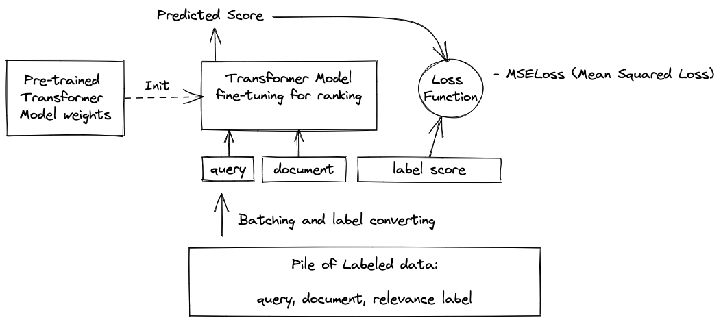
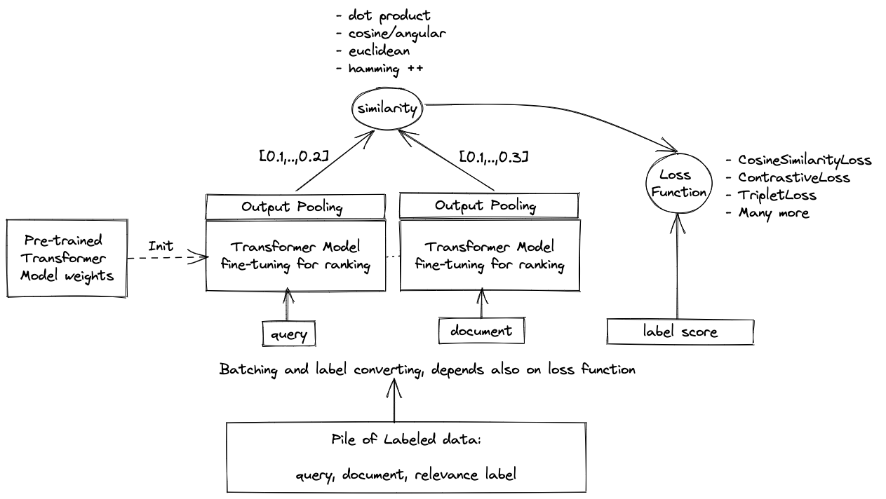
The above figure illustrates the training process; we initialize our model using a pre-trained Transformer. Next, we prepare batches of labeled data of the form <query, document, label>. This data must be pre-processed into a format that the model understands, mapping free text to token ids. As part of this process, we convert the textual graded label representation to a numeric representation using the earlier label gain map. For each batch, the model makes predictions, and the prediction errors are measured using the loss function. The model weights are then adjusted to minimize the loss, one batch at a time.

Once we have trained the model, we can save the model weights and import the model into Vespa for inference and ranking. More on how to represent cross-encoder language models in Vespa will be in a later section in this blog post.

Choosing the Transformer model and model inputs

There are several pre-trained language models based on the Transformer model architecture. Since we operate on English queries and products, we don’t need multilingual capabilities. The following models use the English vocabulary and wordpiece tokenizer.

• bert-base-uncased - About 110M parameters
• MiniLM Distilled model using bert-base-uncased as a teacher, about 22M parameters

Choosing a model is a tradeoff between deployment cost and accuracy. A larger model (with more parameters) will take longer to train and have higher deployment costs but with potentially higher accuracy. In our work, we base our model on weights from a MiniLM model trained on relevancy labels from the MS Marco dataset.

We have worked with the MiniLM models before in our work on MS Marco passage ranking, so we know these models provide a reasonable tradeoff between ranking accuracy and inference efficiency, which impacts deployment cost. In addition, MiniML is a CPU-friendly model, especially with quantized versions. As a result, we are avoiding expensive GPU instances and GPU-related failure modes.

In addition to choosing the pre-trained Transformer model, we must decide which product fields and the order we will input them into the model. Order matters, and the Transformer model architecture has quadratic computational complexity with the input length, so the size of the text inputs significantly impacts inference-related costs.

Some alternative input permutations for our product dataset are:

• query, product title,
• query, product title, brand,
• query, product title, brand, product description,
• query, product title, product description, product bullets.

The product field order matters because the total input length is limited to a maximum of 512 tokens, and shorter input reduces inference costs significantly. Since all products in the dataset have a title, we used only the title as input, avoiding complexity related to concatenating input fields and handling missing fields. Furthermore, product titles are generally longer than, for example, Wikipedia or web page titles.

We trained the model for two epochs, Machine Learning (ML) terminology for two complete iteration over our training examples. Training the model on a free-tier Google Colab GPU takes less than 30 minutes.

Representing cross-encoders in Vespa

Once we have trained our cross-model using the sentence-transformer cross-encoder training library, we need to import it to Vespa for inference and ranking. Vespa supports importing models saved in the ONNX model format and where inference is accelerated using ONNX-Runtime. We export the PyTorch Transformer model representation to ONNX format using an ONNX export utility script. Then we can drop the ONNX file into the Vespa application package and configure how to use it in the product schema:

Model declaration

document product {
    field title type string {..} 
}
field title_tokens type tensor(d0[128]) {
    indexing: input title | embed tokenizer | attribute | summary
}
onnx-model title_cross {
    file: models/title_ranker.onnx
    input input_ids: title_input_ids
    input attention_mask: title_attention_mask
    input token_type_ids: title_token_type_ids
}

The above declares the title_tokens field where we store the subword tokens and the onnx-model with the file name in the application package and its inputs. The title_tokens are declared outside of the document as these fields are populated during indexing.

Using the model in rank-profile

rank-profile cross-title inherits default {
    inputs {
        query(query_tokens) tensor(d0[32])
    }

    function title_input_ids() {
        expression: tokenInputIds(96, query(query_tokens), attribute(title_tokens))
    }

    function title_token_type_ids() {
        expression: tokenTypeIds(96, query(query_tokens), attribute(title_tokens))
    }

    function title_attention_mask() {
        expression: tokenAttentionMask(96, query(query_tokens), attribute(title_tokens)) 
    }

    function cross() {
        expression: onnx(title_cross)({d0:0,d1:0} 
    }
    first-phase {
        expression: cross() 
    }
} 

This defines the rank-profile with the function inputs and where to find the inputs. We cap the sequence at 96 tokens, including special tokens such as CLS and SEP. The onnx(title_cross)({d0:0,d1:0} invokes the model with the inputs and slices the batch dimension (d0) and reads the predicted score.

Vespa provides convenience tensor functions to calculate the three inputs to the Transformer models; tokenInputIds, tokenTypeIds, and tokenAttentionMask. We just need to provide the query tokens and field from which we can read the document tokens. To map text to token_ids using the fixed vocabulary associated with the model, we use Vespa’s support for wordpiece embedding. This avoids document side tokenization at inference time, and we can just read the product tokens during ranking. See the full product schema.

Neural Bi-Encoder using pre-trained language models

Another popular approach for neural ranking is the two-tower or bi-encoder approach. This approach encodes queries and documents independently.

For text ranking, queries and documents are encoded into a dense embedding vector space using one or two Transformer models. Most methods use the same Transformer instance, but it’s possible to decouple them. For example, suppose both towers map documents and queries to the same vector dimensionality. In that case, one could choose a smaller Transformer model for the online query encoder versus the document tower to reduce latency and deployment costs.

The model learns the embedding vector representation from the labeled training examples. After training the model, one can compute the embeddings for all products, index them in Vespa, and use a nearest-neighbor search algorithm at query time for efficient document retrieval or ranking. In this work, Amazon has provided the “retrieved” products for all queries, so we don’t need HNSW indexing for efficient approximate nearest neighbor search.

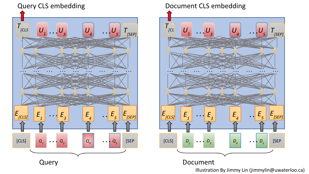
The above illustrates the bi-encoder approach. This illustration uses the Transformer CLS (classification token) output and uses that as the single dense vector representation. Another common output pooling strategy is calculating the mean over all the token vector outputs. Other representation methods use multiple vectors to represent queries and documents. One example is the ColBERT model described in this blog post.

The above illustrates training a bi-encoder for semantic similarity. Training bi-encoders for semantic similarity or semantic search/retrieval/ranking has more options than training cross-encoders.

As with the cross-encoder, we must select a pre-trained model, minding size and quality.

The model size impacts quality, inference speed, and vector representation dimensionality. For example, bert-base-uncased uses 768 dimensions, while MiniLM uses 384. Lower dimensionality lowers the computational complexity of the similarity calculations and reduces the embedding storage footprint.

Furthermore, how we batch the input training data, the vector similarity function, and, most importantly, the loss function determines the quality of the model on the given task. While loss functions are out of the scope of this blog post, we would like to mention that training a bi-encoder for semantic retrieval over a large corpus, which “sees” many irrelevant documents, needs a different loss function than a bi-encoder model used for re-ranking.

Like with the cross-encoder, we must decide what product fields we encode. Instead of inputting multiple product fields, we train two bi-encoder models, one that uses the product title and another that encodes the description. Both models are based on sentence-transformers/all-MiniLM-L6-v2.

Representing bi-encoders in Vespa

A single Vespa document schema can contain multiple document embedding fields,

document product {
    field title type string {}
    field description type string {}
}
field title_embedding type tensor(d0[384]) {
    indexing: input title | embed title | attribute | summary
    attribute {
        distance-metric: angular 
    }
}
field description_embedding type tensor(d0[384]) {
    indexing: input description | embed description | attribute | summary
    attribute {
        distance-metric: angular 
    }
}

We declare two indexed tensors and use use Vespa’s support for embedding bi-encoder models, see text embeddings made easy. Both query and document-side embeddings can be produced within the Vespa cluster, not having to rely on external embedding services. See the full product schema.

Evaluation

The official dataset evaluation metric is NDCG (Normalized Discounted Cumulative Gain), a precision-oriented metric commonly used for ranking datasets with graded relevance judgments.

An important observation is that the task only considers the ranking of products with judgment labels. In other words, we can assume that a perfect magic retriever has retrieved all relevant documents (plus irrelevant documents).

Results

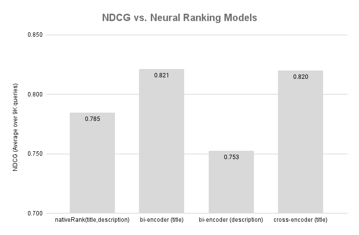
The above figure summarizes the NDCG scores for our three neural ranking models. We also include a zero-shot baseline model from the last blog post.

The bi-encoder and cross-encoder using the product title performed better than all the zero-shot models from the previous post. However, the bi-encoder trained on the description performs worse than our lexical baselines. This result demonstrates that not all text vectorization models perform better than lexical ranking models, even when fine-tuned on the domain. We did not pre-process the description, like HTML stripping or other data cleaning techniques, which might have impacted the ranking results. We did not expect the bi-encoder to perform similarly to the cross-encoder; the latter is a more advanced ranking method, with both the query and the product title fed into the model.

Understanding that these NDCG results are from about 20 products per query is essential. Re-ranking is a more straightforward task than retrieval, and the downside is limited as we have relatively few products to re-rank per query. In a later post in this series, we focus on learning to retrieve, comparing it with learning to rank, as there are subtle differences.

Summary

This blog post introduced two popular neural ranking methods. We evaluated their performance on the test split and reported their ranking results. We have open-sourced this work as a Vespa sample application, and you can reproduce the neural training routine using this notebook .

Next Blog

In the next post in this series, we will deep dive into classic learning to rank using listwise ranking optimization with Lambdarank and Gradient Boosting (GB). GB models are famous for their performance on tabular data and are prevalent in e-commerce search ranking. We will also describe how to use a combination of lexical, statistical, and neural features and feed them into the GB model. Lastly, for run-time inference and ranking, we will use Vespa’s support for LightGBM and XGBoost models, two popular frameworks for training GBDT models.