Photo by Jukan Tateisi on Unsplash

Imagine you have a machine-learned model that you would like to use in some application, for instance, a transformer model to generate vector representations from text. You measure the time it takes for a single model evaluation. Then, satisfied that the model can be evaluated quickly enough, you deploy this model to production in some model server. Traffic increases, and suddenly the model is executing much slower and can’t sustain the expected traffic at all, severely missing SLAs. What could have happened?

You see, most libraries and platforms for evaluating machine-learned models are by default tuned to use all available resources on the machine for model inference. This means parallel execution utilizing a number of threads equal to the number of available cores, or CPUs, on the machine. This is great for a single model evaluation.

Unfortunately, this breaks down for concurrent evaluations. This is an under-communicated and important point.

Let’s take a look at what happens. In the following, we serve a transformer model using Vespa.ai. Vespa is a highly performant and web-scalable open-source platform for applications that perform real-time data processing over large data sets. Vespa.ai uses ONNX Runtime under the hood for model acceleration. We’ll use the original BERT-base model, a 12-layer, 109 million parameter transformer neural network. We test the performance of this model on a 32-core Xeon Gold 2.6GHz machine. Initially, this model can be evaluated on this particular machine in around 24 milliseconds.

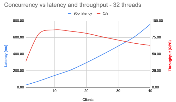
Here, the blue line is the 95th percentile latency, meaning that 95% of all requests have latency lower than this. The red line is the throughput: the requests per second the machine can handle. The horizontal axis is the number of concurrent connections (clients).

As the number of simultaneous connections increases, the latency increases drastically. The maximum throughput is reached at around 10 concurrent requests. At that point, the 95th percentile latency is around 150ms, pretty far off from the expected 24ms. The result is a highly variable and poor experience.

The type of application dictates the optimal balance between low latency and high throughput. For instance, if the model is used for an end-user query, (predictably) low latency is important for a given level of expected traffic. On the other hand, if the model generates embeddings before ingestion in some data store, high throughput might be more important. The driving force for both is cost: how much hardware is needed to support the required throughput. As an extreme example, if your application serves 10 000 queries per second with a 95% latency requirement of 50ms, you would need around 200 machines with the setup above.

Of course, if you expect only a minimal amount of traffic, this might be totally fine. However, if you are scaling up to thousands of requests per second, this is a real problem. So, we’ll see what we can do to scale this up in the following.

Parallel execution of models

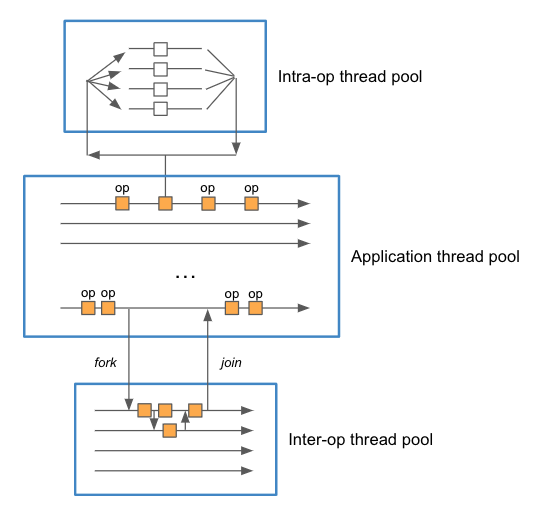
We need to explain the threading model used during model inference to see what is happening here. In general, there are 3 types of threads: inference (application), inter-operation, and intra-operation threads. This is a common feature among multiple frameworks, such as TensorFlow, PyTorch, and ONNX Runtime.

The inference threads are the threads of the main application. Each request gets handled in its own inference thread, which is ultimately responsible for delivering the result of the model evaluation given the request.

The intra-operation threads evaluate single operations with multi-threaded implementations. This is useful for many operations, such as element-wise operations on large tensors, general matrix multiplications, embedding lookups, and so on. Also, many frameworks chunk together several operations into a higher-level one that can be executed in parallel for performance.

The inter-operation threads are used to evaluate independent parts of the model in parallel. For instance, a model containing two distinct paths joined in the end might benefit from this form of parallel execution. Examples are Wide and Deep models or two-tower encoder architectures.

In the example above, which uses ONNX Runtime, the default disables the inter-operation threads. However, the number of intra-operation threads is equal to the number of CPUs on the machine. In this case, 32. So, each concurrent request is handled in its own inference thread. Some operations, however, are executed in parallel by employing threads from the intra-operation thread pool. Since this pool is shared between requests, concurrent requests need to wait for available threads to progress in the execution. This is why the latency increases.

The model contains operations that are run both sequentially and in parallel. That is why throughput increases to a certain level even as latency increases. After that, however, throughput starts decreasing as we have a situation where more threads are performing CPU-bound work than physical cores in the machine. This is obviously detrimental to performance due to excessive thread swapping.

Scaling up

To avoid this thread over-subscription, we can ensure that each model runs sequentially in its own inference thread. This avoids the competition between concurrent evaluations for the intra-op threads. Unfortunately, it also avoids the benefits of speeding up a single model evaluation using parallel execution.

Let’s see what happens when we set the number of intra-op threads to 1.

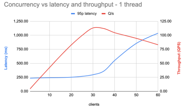
As seen, the latency is relatively stable up to a concurrency equalling the number of cores on the machine (around 32). After that, latency increases due to the greater number of threads than actual cores to execute them. The throughput also increases to this point, reaching a maximum of around 120 requests per second, which is a 40% improvement. However, the 95th percentile latency is now around 250ms, far from expectations.

So, the model that initially seemed promising might not be suitable for efficient serving after all.

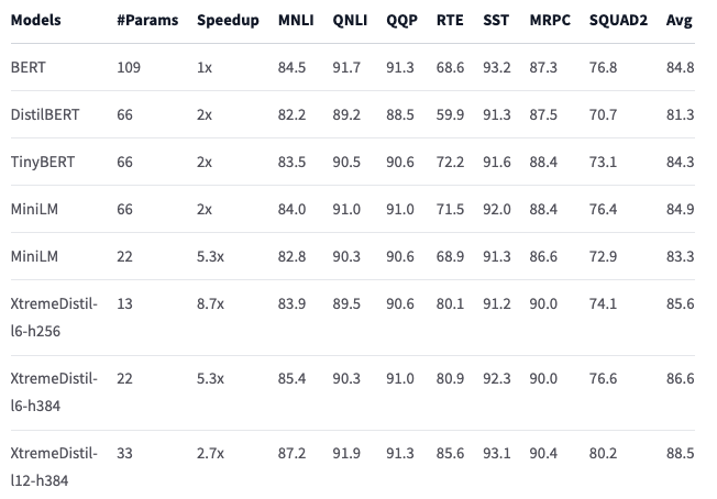
The first generation of transformer models, like BERT-base used above, are relatively large and slow to evaluate. As a result, more efficient models that can be used as drop-in replacements using the same tokenizer and vocabulary have been developed. One example is the XtremeDistilTransformers family. These are distilled from BERT and have similar accuracy as BERT-base on many different tasks with significantly lower computational complexity.

In the following, we will use the XtremeDistil-l6-h256 model, which only has around 13M parameters compared to BERT-base’s 109M. Despite having only 12% of the parameter count, the accuracy of this model is very comparable to the full BERT-base model:

Using the default number of threads (same as available on the system), this model can be evaluated on the CPU is around 4ms. However, it still suffers from the same scaling issue as above with multiple concurrent requests. So, let’s see how this scales with concurrent requests with single-threaded execution:

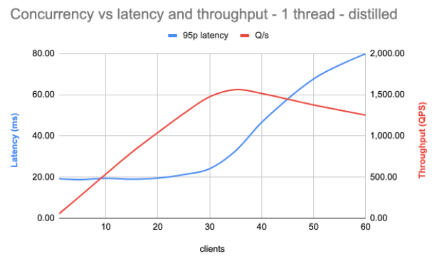
As expected, the latency is much more stable until we reach concurrency levels equalling the number of cores on the machine. This gives a much better and predictable experience. The throughput now tops out at around 1600 requests per second, vastly superior to the other model, which topped out at roughly 120 requests per second. This results in much less hardware needed to achieve wanted levels of performance.

Experiment details

To measure the effects of scaling, we’ve used Vespa.ai, an open-source platform for building applications that do real-time data processing over large data sets. Designed to be highly performant and web-scalable, it is used for diverse tasks such as search, personalization, recommendation, ads, auto-complete, image and similarity search, comment ranking, and even finding love.

Vespa.ai has many integrated features and supports many use cases right out of the box. Thus, it offers a simplified path to deployment in production without the complexity of maintaining many different subsystems. We’ve used Vespa.ai as an easy-to-use model server in this post. In Vespa.ai, it is straightforward to tune the threading model to use for each model:

<model-evaluation>
  <onnx>
    <models>
      <model name="reranker_margin_loss_v4">
        <intraop-threads> number </intraop-threads>
        <interop-threads> number </interop-threads>
        <execution-mode> parallel | sequential </execution-mode>
      </model>
    </models>
  </onnx>
</model-evaluation>

Also, it is easy to scale out horizontally to use additional nodes for model evaluation. We have not explored that in this post.

The data in this post has been collected using Vespa’s fbench tool, which drives load to a system for benchmarking. Fbench provides detailed and accurate information on how well the system manages the workload.

Summary

In this post, we’ve seen that the default thread settings are not suitable for model serving in production, particularly for applications with a high degree of concurrent requests. The competition for available threads between parallel model evaluations leads to thread oversubscription and performance suffers. The latency also becomes highly variable.

The problem is the shared intra-operation thread pool. Perhaps a different threading model should be considered, which allows for utilizing multiple threads in low traffic situations, but degrades to sequential evaluation when high concurrency is required.

Currently however, the solution is to ensure that models are running in their own threads. To manage the increased latency, we turned to model distillation, which effectively lowers the computational complexity without sacrificing accuracy. There are additional optimizations available which we did not touch upon here, such as model quantization. Another one that is important for transformer models is limiting input length as evaluation time is quadratic to the input length.

We have not considered GPU evaluation here, which can significantly accelerate execution. However, cost at scale is a genuine concern here as well.

The under-communicated point here is that platforms that promise very low latencies for inference are only telling part of the story. As an example, consider a platform promising 1ms latency for a given model. Naively, this can support 1000 queries per second. However, consider what happens if 1000 requests arrive at almost the same time: the last request would have had to wait almost 1 second before returning. This is far off from the expected 1ms.