How we implemented a production-ready question-answering application and reduced response time by more than two orders of magnitude.

Imagine you’ve created a machine learning system that surpasses state-of-the-art performance on some task. You’ve optimized for a set of objectives like classification accuracy, F1 scores, or AUC. Now you want to create a web service from it. Other objectives, such as the time or cost of delivering a result to the user, become more important.

These two sets of objectives are typically in conflict. More accurate models are often large and computationally expensive to evaluate. Various optimizations like reducing the models’ precision and complexity are often introduced to use such models in production. While beneficial for decreasing cost and energy consumption, this, unfortunately, hurts accuracy.

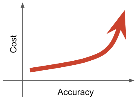
Obviously, inference time can be drastically lowered if accuracy is not important. Likewise, accurate responses can be produced at high cost. Which solution to ultimately choose lies somewhere between these extremes. A useful technique for selecting the best solution is to enumerate them in terms of accuracy and cost. The set of solutions not dominated by others is called the Pareto frontier and identifies the best trade-offs between accuracy and cost.

In a previous blog post, we introduced a serving system that reproduces state-of-the-art accuracy in open-domain question-answering. We based this on Facebook’s Dense Passage Retrieval (DPR), which is a Python-based research system. We built the serving system using Vespa.ai, the open-source big data serving engine, which is uniquely suited to tasks like this due to its native support for fast similarity search and machine learned models in search and ranking. The result is a web service taking a single question and returning an exact answer.

While this system reproduced DPR’s result and thus had excellent accuracy metrics, the response time was initially poor, as measured in end-to-end latency. This post will describe the various optimizations we made to bring performance to acceptable levels for a production system.

Vespa.ai is built for production and thus has quite a few options for serving time optimizations. We will particularly use Vespa.ai’s ability to retrieve and rank documents using multiple worker threads per query to significant effect. However, this application’s main cost is in evaluating two BERT models. One of the questions we would like to answer is whether smaller models with full precision are preferable to larger models with quantized parameters. We’ll develop the Pareto frontier to evaluate the merits of the various optimizations.

We’ll start with an overview of the serving system and identify which parts of the system initially drive the cost. For more details on the implementation, we refer to the previous blog post in this series.

Question Answering

The system’s task is to produce a textual answer in response to a question given in natural language. There are primarily three stages involved:

• The encoder generates a representation vector for the question.
• The retriever performs a nearest neighbor search among the 21 million indexed passages.
• The reader finds the most relevant passage and extracts the final answer.

The following figure illustrates the process:

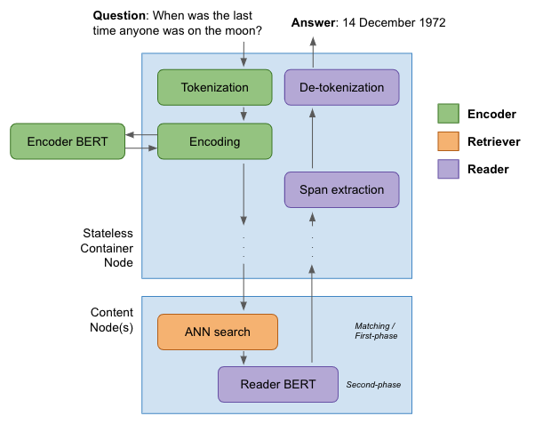
The encoder first creates a tokenized representation from the question. This vector of token IDs is sent as input to the encoder BERT model. This is initially a standard BERT-base model with 12 layers and a hidden layer size of

1. The final hidden layer state is used as a representation vector for the question. As seen in the figure above, this primarily happens in the stateless container layer in Vespa. The token and vector representation is passed down (“scattered”) to all content nodes to perform the query.

On the content nodes, the passages have been indexed with their own representation vectors. These vectors have been constructed so that the euclidean distance between question and passage vectors indicate similarity. This is used in the HNSW algorithm to perform an approximate nearest neighbor search. The 10 passages with the smallest euclidean distance are sent to the next stage.

The second-phase ranking stage, also performed on each content node, evaluates the reader BERT model. Like the encoder model, this is initially a BERT-base model with 12 layers and hidden length 768. The token representations from the query and each passage are combined to form the model input. The reader model produces three probability scores: the relevance score and the start and end indices of the answer in the passage’s token sequence. The passage with the best relevance score is selected as the winner, and its token representation is returned to the stateless layer. There, custom code extracts the best span using the start and end indices, de-tokenizes it, and returns the resulting textual answer.

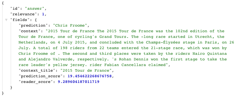
Now, that’s a lot of work. Here is an example of a response to the question “Who won Tour De France in 2015”, where the most relevant passage is retrieved and the correct answer “Chris Froome” is extracted:

To measure performance, we deployed the system on a single machine with an Intel Xeon Gold 6240 processor with 200 GB RAM and SSD disk. We evaluate the system over 3610 questions and record the average latency and exact-match score. Initially, the system achieves an exact-match score of 40.64. Before any consideration has been made to optimize performance, the time spent in the three stages mentioned above is:

• Encoding model: 300 ms
• Approximate nearest neighbor search: 13 ms
• Top-10 reader ranking: 9085 ms

Obviously, a total end-to-end latency of 9.4 seconds is not anything close to acceptable as a service. In the following, we’ll lower this to well below 100 ms.

Multi-threaded retrieval ranking

Initially, the most expensive step by far is the reader stage. By default, Vespa does all ranking for a query on a single thread. This is a reasonable default to maximize throughput when the computational cost is low. In this case, this means that the reader model is evaluated - in sequence - for each of the top 10 passages. This results in high query latency.

However, Vespa has an option of using multiple threads per search. Setting this value brings the average end-to-end latency down to 2.04 seconds, a more than 4x improvement without affecting the exact match score.

It is worth clarifying that the reader model is not evaluated batch-wise. This is due to Vespa’s ranking framework, where ranking expressions score a single passage and query pair. For BERT models, however, this is not significant as evaluation time is linear with batch size. One reason is tensor multiplications with tensors of 3 or more dimensions, as these iterate over several hardware-optimized matrix-matrix multiplications anyway.

In general, Vespa has many options to tune performance, such as easily distributing the workload on additional content nodes. While we don’t explore that here, see the Vespa serving scaling guide for more information.

Token sequence length

One of the defining and most prominent features of BERT models is the full-attention layer. While this was a significant breakthrough in language understanding, it has an unfortunate O(n^2) effect on evaluation time.

So, the length of the token sequence input to the BERT model significantly impacts inference time. Initially, the encoder BERT model had an input length of 128. By reducing it to 30, we decrease inference time from 300 ms to 125 ms without loss of accuracy.

Likewise, the reader model initially had an input length of 380. By reducing this to 128, we reduce average latency from 1.9 seconds to 741 ms, a significant reduction. However, we do get a decrease in accuracy, as some question and passage combinations can result in token sequences longer than 128. This reduced the exact match score to 39.61.

Both the encoder and reader model support dynamic length inputs, but Vespa currently only supports fixed length inputs. This will be fixed in the near future, however. In summary, shortening token input lengths of the encoder and reader models result in a 3x speedup.

Model quantization

Neural network models are commonly trained using single-precision floating-point numbers. However, for inference in production, it has been shown that this level of precision is not always necessary. The parameters can be converted to a much smaller integer representation without significant loss in accuracy. Converting the parameters from a 32-bit floating-point to 8-bit integers reduces the model size by 75%. More importantly, integer operations execute much faster. Modern CPUs that support AVX512 Vector Neural Network Instructions (VNNI) are designed to accelerate INT8 inference performance. Additionally, evaluating such quantized models requires less power.

Quantizing the reader model brings its size down from 435Mb to 109Mb. The latency for the system drops on average to 374 ms. This has a slightly unfortunate effect on accuracy, dropping the exact match to 37.98. Likewise, quantizing the encoder model results in a similar size reduction, and system evaluation time drops to 284 ms. The exact-match score drops to 37.87.

In summary, model quantization of both reader and encoder models result in another 3x speedup.

Miniature models

Until this point, both the encoder and reader models are based on pre-trained BERT-base models, containing 12 layers with hidden dimension size of 768 and thus around 110 million parameters. These are reasonably large models, particularly when used in time-constrained environments. However, in the paper Well-Read Students Learn Better: On the Importance of Pre-training Compact Models, the authors show that smaller models can indeed work well. The “miniature” models referenced in this paper can be found in the Transformers model repository.

We trained new reader models as described in the DPR repository, basing them on the following pre-trained BERT miniature models:

• Medium (8 layers, 512 hidden size)
• Small (4 layers, 512 hidden size)
• Mini (4 layers, 256 hidden size)
• Tiny (2 layers, 128 hidden size)

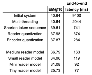
We also quantize each model. The full overview of all 20 models (5 reader models, with and without quantization, with and without quantized encoder model) with exact match scores and average latency is given in the table below:

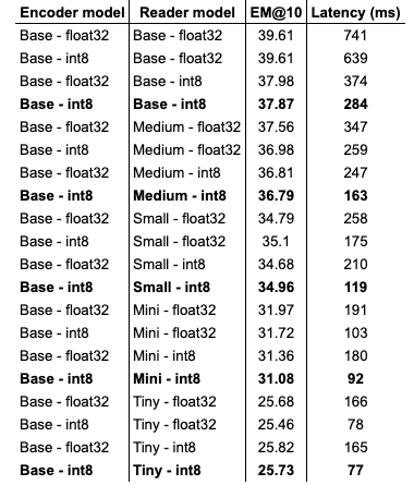
Plotting these results:

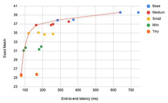
In the figure above, the red line represents the Pareto front. The points along this front are also marked in bold in the table above. Recall that these points represent the best trade-offs between exact match and latency, meaning that there are no other points that are superior in both exact match and latency for each point along this front.

One interesting result that can be seen here is that, in general, quantized models dominate other models with higher precision. For instance, the medium quantized model has better exact match and latency numbers than the small models with higher precision. So, in this case, even though quantization reduces accuracy, it is more beneficial to choose a large model that has been quantized over a smaller model that has not.

The Pareto front visualizes the objectively best solutions, and our subjective preferences would guide us in finding the optimal solution. The tests above have been run on a single Intel Xeon Gold 6240 machine. More powerful processors would lower the overall latency numbers but not change the overall shape. The exact solution to choose is then based on our latency and hardware budgets. For instance, organizations with considerable resources that can scale up sufficiently can justify moving to the right on this front. The economy of scale can mitigate the cost of hardware investments and energy consumption to make the service viable. Such a solution might be out of reach for others.

Conclusion

In summary, we’ve taken a research application with poor performance to levels suitable for production. From 9.4 seconds for the full model down to 70ms for the tiny model, this represents a 130x speedup. Unfortunately, to get down to these levels, we noted a significant drop in exact-match as well. The best choice lies somewhere between these extremes. If we were to bring this application into production, we could use more powerful hardware to bring the latency below 100ms with acceptable exact match metrics.

There are quite a few optimizations we didn’t try that are outside the scope of this article. For instance, FastFormers: Highly Efficient Transformer Models for Natural Language Understanding includes some additional optimizations for more efficient inference such as model pruning. Also, new generations of BERT models attempt to alleviate the performance problems associated with the full-attention mechanism. For instance, the Big Bird architecture seems promising.

We omitted training miniature encoder models. From a latency point of view, using the miniature BERT models in question encoding have an additional benefit as the vector representation for the question and passages are shorter. Thus the approximate nearest neighbor search would become more efficient. However, this would likely result in a significant drop in accuracy and the time spent in the ANN is not a significant driver of latency anyway.

Adding additional content nodes would allow for distributing the workload. This would likely not reduce latency but would increase the number of passages we can evaluate with the reader model. We will return to this in an upcoming blog post.