Photo by Graham Holtshausen on Unsplash

The first blog post on billion-scale vector search covered methods for compressing real-valued vectors to binary representations and using hamming distance for efficient coarse level search. The second post described approximate nearest neighbor search tradeoffs using Hierarchical Navigable Small World (HNSW), including memory usage, vector indexing performance, and query performance versus accuracy.

This post in this series on billion scale search introduces a cost-efficient hybrid method for approximate nearest neighbor (ANN) search combining (HNSW) with disk-backed inverted file. We name this hybrid method for ANN search for HNSW-IF.

Introduction

In-memory algorithms, like HNSW, for approximate nearest neighbor search, offer fast, high accuracy vector search but quickly become expensive for massive vector datasets due to memory requirements. The HNSW algorithm requires storing the vector data in memory for low latency access during query and indexing.

For example, a billion scale vector dataset using 768 dimensions with float precision requires close to 3TiB of memory. In addition, the HNSW graph data structure needs to be in-memory, which adds 20-40% in addition to the vector data. Given this, indexing a 1B vector dataset using HNSW will need about 4TiB of memory.

In 2022, many cloud providers offer cloud instance types with large amounts of memory, but these instance types also come with many v-CPUs, which drives production deployment costs. These high-memory and high-compute instance types support massive queries per second and might be the optimal instance type for applications needing to support large query throughput with high recall. However, many real-world applications using vector search do not need enormous query throughput but still need to search large billion-scale vector datasets with relatively low latency with high accuracy. Therefore, large cloud instance types with thousands of GiB of memory and hundreds of v-CPUs are not cost-efficient for those low query volume use cases.

Due to this, there is an increasing interest in hybrid ANN search solutions using solid-state disks (SSD) to store most of the vector data combined with in-memory graph data structures. SPANN: Highly-efficient Billion-scale Approximate Nearest Neighbor Search introduces a simple and effective solution for hybrid ANN search.

Introducing SPANN

SPANN combines the graph-based in-memory method for ANN search with the inverted file using clustering.
SPANN partitions the vector dataset of M vectors into N clusters. The paper explores setting N to a number between 4% to 20% of M. A centroid vector represents each cluster. The paper describes different algorithms for clustering the vector dataset into N clusters and finds that hierarchical balanced clustering (HBC) works best. See Figure 10 in the paper: Different types of centroid selection.

The cluster centroid vector points to a posting list containing the vectors close to the cluster centroid. Disk-based data structures back the posting lists of non-centroids, and centroids are indexed using an in-memory ANN search algorithm. Unlike quantization techniques for ANN search, all vector distance calculations are performed with the full-precision vector representation.

SPANN searches for the k closest centroid vectors of the query vector in the in-memory ANN search data structure. Then, it reads the k associated posting lists for the retrieved centroids and computes the distance between the query vector and the vector data read from the posting list.

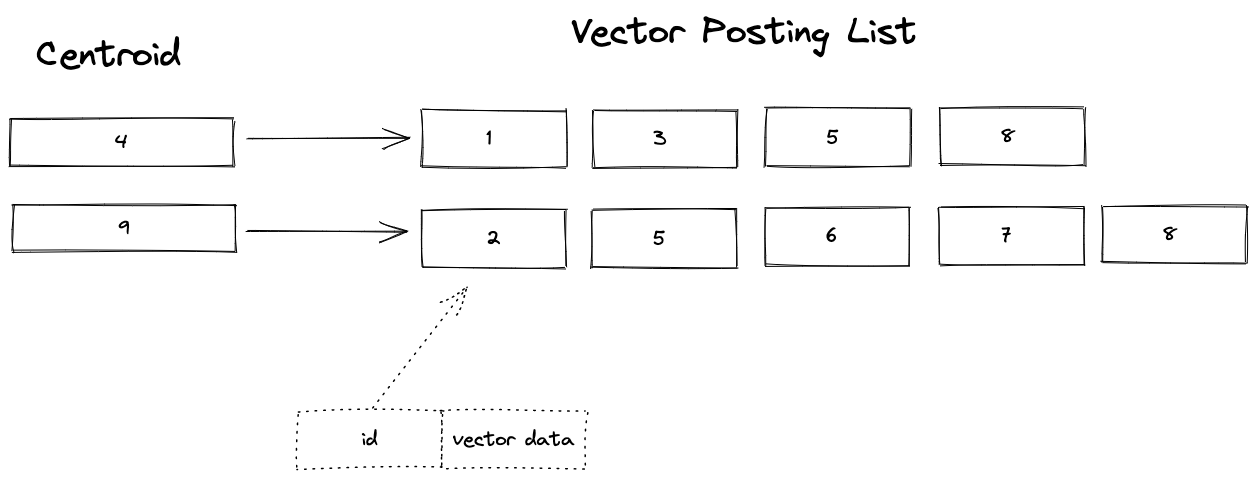Figure 1 illustrates SPANN.

Figure 1 gives a conceptual overview of SPANN for a small vector dataset of ten vectors. There are two centroid vectors, vectors 4 and 9, referencing a posting list consisting of the vectors close to the cluster the centroid represents. A vector might be close to multiple cluster centroids, for example, vector 5 and vector 8 in the figure above. These are examples of boundary vectors that lay in between multiple centroids.

The offline clustering part of SPANN tries to balance the clusters so that the posting lists are equal in size to reduce the time it takes to read the posting list from disk. For example, if the vector has 100 dimensions using int8 precision and int32 for the vector id, each posting list entry uses 104 bytes. With a 4KiB disk read page size, one can read 1024 posting entries in a single IO read operation.

Hybrid HNSW-IF with Vespa

Inspired by the SPANN paper, we at the Vespa team implemented a simplified version of SPANN using Vespa primitives, released as a Vespa sample application. We call this hybrid ANN search method for HNSW-IF.

Vespa features used to implement HNSW-IF:

• Real-time HNSW vector indexing
• Real-time inverted index data structures
• Disk based vectors using Vespa dense tensor type using paged option
• Phased ranking
• Stateless search and document processors

The following sections outline the differences between the method described in the SPANN paper and the Vespa HNSW-IF sample application implementation using Vespa primitives.

Vector Indexing and Serving architecture

• Instead of clustering and computing centroids offline, let vectors from the original dataset represent centroids and use the original vector id as the centroid id. This approach does not waste any distance calculations at query time as the centroids are valid eligible vectors. A subset of the vector dataset (20%) is selected randomly to represent centroids. Random centroid selection only requires one pass through the vector dataset, splitting the dataset into centroids and non-centroids.

• The vectors representing centroids are indexed in memory using Vespa’s support for vector indexing using Hierarchical Navigable Small World (HNSW). Searching 200M centroid vectors indexed with HNSW typically takes 2-3 milliseconds, single-threaded (depending on recall target and HNSW settings). Both the graph data structure and the vector data are stored in memory.

• During indexing of vectors that are not cluster centroids, search for the k closest centroids in the HNSW graph of centroids and index the closest centroid ids using Vespa’s support for inverted indexes. Later, when the index build is complete, a search for a centroid id efficiently retrieves the closest non-centroid vector id. The inverted index consists of a dictionary of centroid ids pointing to posting lists of non-centroid vector ids. For a given billion scale dataset with 20% centroids, the maximum centroid dictionary vocabulary size is 200M.

• A non-centroid vector might be present in multiple centroid clusters. Instead of storing the vector data in the posting lists, the vector data is stored in a separate Vespa data structure and avoids duplication caused by storing the same vector data in multiple posting lists. Instead, the Vespa posting list entry stores the closeness (inverted distance) of the vector to the centroid, scaled to integer weight. Only the vector ids are duplicated across centroid posting lists, not the vector data itself. Vespa posting lists are compressed using standard techniques for lossless posting list compression.

Querying Vectors

For an input query vector, first search the vectors representing centroids, using HNSW, for the k closest centroids. Next, using the retrieved k nearest centroids from HNSW search, search the inverted index using logical disjunction (OR) of the centroid ids retrieved by the HNSW graph search. The actual implementation uses the Vespa dotProduct multivalued query operator.

Each node involved in the inverted index query ranks the retrieved non-centroid vectors by calculating the distance between the vector and the query vector. Finally, the result of the two searches is merged and returned.

The query serving flow can be optimized by two heuristics:

• Cluster centroid dynamic pruning. After retrieving the k closest centroids from searching the HNSW graph, distant centroids (compared to the nearest centroid) can be pruned without significantly impacting recall. This distant centroid pruning heuristic reduces the number of seeks and reads for the inverted index query evaluation. The centroid pruning heuristic is dynamic; a query vector that retrieves many equally close centroids allows little pruning, while a query vector that retrieves centroids with more considerable distance differences might allow pruning many.

• Retrieve using dynamic pruning. This heuristic sorts the retrieved vector ids by the closeness(q, centroid) * closeness(centroid, v) transitive closeness score where q is the query vector and v is the document vector. This phase is implemented as a Vespa first-phase ranking phase. The closeness(centroid,v) weight is stored in the posting list, and the closeness(q, centroid) is passed as a query term weight with the dotProduct query operator. This heuristic enables limiting the number of vector page-ins by using Vespa’s support for controlling phased ranking. The local per node second-phase ranking calculates the full precision, (closeness(q,v), which involves paging the vector data into memory from disk. The maximum re-ranking depth is a query time hyperparameter enabling easy experimentation.

Real-world considerations

Real-world applications using vector search need both batch and real-time vector indexing:

• Batch indexing: An embedder model (for example, Data2Vec) that maps data to vector representation is trained, and embedding vector representations are produced for all known data items.
• Incremental Real-time indexing: A new data item arrives and is encoded with the current version of the embedder model and needs to be indexed.

In addition, data items (with vector representation) need to be updated and deleted. The hybrid method described in this blog post supports all CRUD (Create, Read, Update, Delete) operations using the standard Vespa APIs.

• Batch indexing with a new embedder model is handled by adding a model version field to the schema. Serving queries must restrict the search for vectors to the given model id using standard inverted index query evaluation and constrained vector search. See Query Time Constrained Approximate Nearest Neighbor Search and Embedding model hot swap. Having multiple active model versions increases the storage-related deployment cost linearly with the number of models.

• New vectors using an existing embedding model are added as a non-centroid vector. As long as the ratio of centroids is large, one can expect to grow the vector volume significantly without significantly degrading accuracy.

The only thing the application owner needs to consider is that deleting large amounts of centroid vectors will negatively impact recall. For most large-scale vector use cases, this is not a real problem. If the use case requires deleting many vector items, one can consider decoupling centroids from real vectors so that centroids are real centroids and not vectors part of the dataset.

Vespa Experimental Setup

The following section describes our experiments with the Vespa HNSW-IF sample application using Vespa Cloud’s performance environment. The Vespa Cloud performance environment makes it easy to iteratively develop applications and choose the ideal instance types for any size vector dataset.

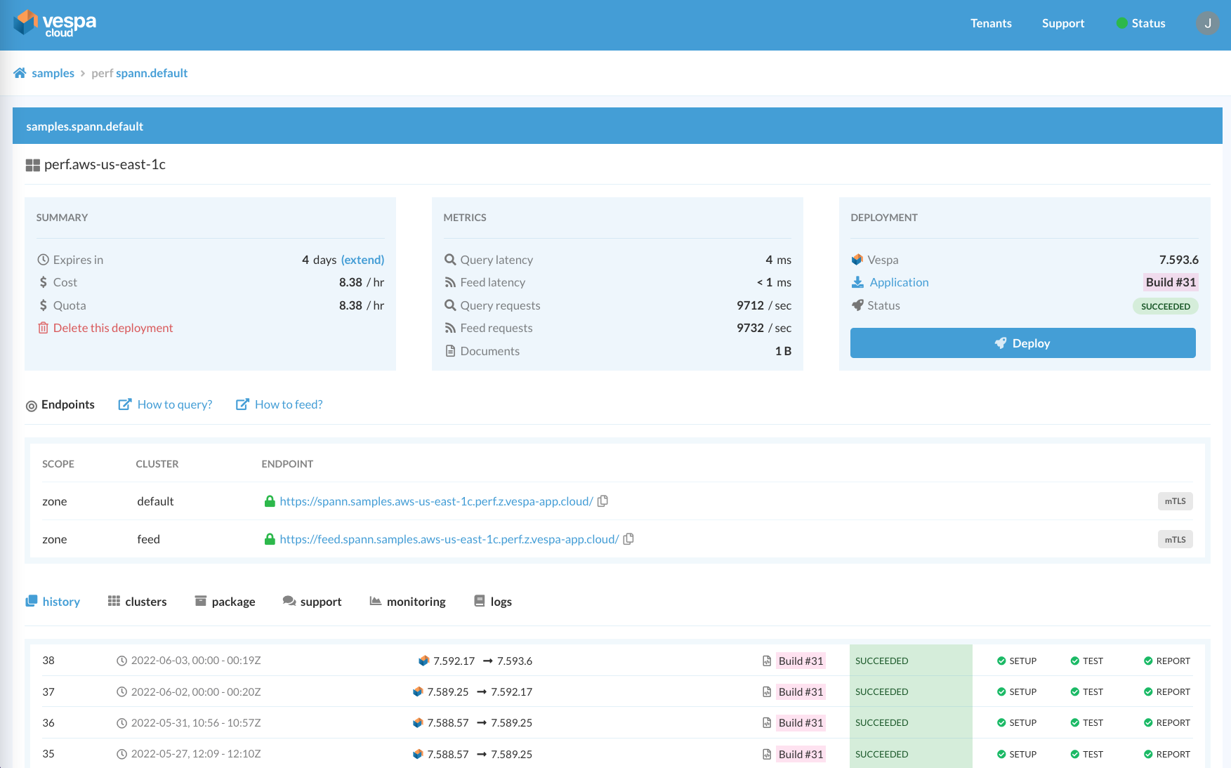Vespa Cloud Console - sample app deployment in Vespa Cloud perf environment in aws-us-east-1c region.

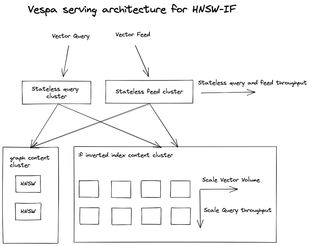Vespa HNSW-IF serving architecture overview.

The Vespa HNSW-IF representation uses the same Vespa document schema to represent centroid and non-centroid vectors. They are differentiated using a single field of type bool.

Using two content clusters with the same document schema enables using different instance types for the two vector types:

• High memory instances with remote storage for the centroid vectors using in-memory HNSW.
• Inexpensive low memory instances with fast local storage for the non-centroid vectors.

This optimizes the deployment and resource cost - the vectors indexed using HNSW does not need fast local disks since queries will never page data from disk during queries. Similarly, for vectors indexed using inverted file, the instances don’t need an awful amount of memory, but more memory can improve query performance due to page caching.

The Vespa inverted index posting lists do not contain the vector data. Instead, vector data is stored using Vespa paged tensor attributes, a type of disk-backed memory mapped forward-index. The downside of not storing the vector data in the postings file is that paging in a vector from disk for distance calculation requires one additional disk seek. However, in our experience, locally attached SSD disks are rarely limited by random seek but by GiB/s throughput bandwidth.

Vector Dataset

For our experiments with HNSW-IF, we use the 1B Microsoft SPACEV-1B vector dataset:

Microsoft SPACEV-1B is a new web search-related dataset released by Microsoft Bing for this competition. It consists of document and query vectors encoded by the Microsoft SpaceV Superior model to capture generic intent representation.

The SPACEV-1B vector dataset consists of 1-Billion 100-dimensional vectors using int8 precision and 29,3K queries with 100 ground truth (exact neighbors) per query. The distance-metric used for the dataset is euclidean which is the default Vespa nearest neighbor search distance-metric. The dataset’s ground truth neighbors are used to evaluate the accuracy (recall) of the hybrid HNSW-IF approach.

Vespa Schema

The sample application uses the following Vespa document schema. Supported Vespa schema field types include string, long, int, float, double, geo position, bool, byte, and tensor fields. Vespa’s first-order dense tensor fields represent vector fields. Vespa’s tensor fields support different tensor cell precision types, including int8, bfloat16, float, and double for real-valued vectors. The SPACEV-1B vector dataset uses int8 precision.

schema vector {

  document vector {

    field id type int {}

    field vector type tensor<int8>(x[100]) {
      indexing: attribute | index
    }

    field neighbors type weightedset<string> {
      indexing: summary | index
    }

    field disk_vector type tensor<int8>(x[100]) {
      indexing: attribute
      attribute: paged
    }

    field in_graph type bool {}
  }
}

Vespa vector document schema. See full version

The random centroid selection is performed outside of Vespa using a python script that reads the input vector data file and randomly selects 20% to represent centroids and sets the in_graph field of type bool to true and populate the vector field with the vector data. The feeder feeds the vector data with in_graph set to true first, to populate the graph content cluster using HNSW indexing, before feeding the non-centroid vectors.

The neighbors field is of type weightedset<string>. The weightedset<string>type allows mapping a string key (the centroid id in this case) to an integer weight. This field is populated by a custom document processor which searches the HNSW graph when feeding non-centroid vectors with in_graph set to false.

For example, for vector 8 from figure 1, the field would be populated with two centroids found from searching the HNSW graph:

{
    "put": "id:spann:vector::8"
    "fields": {
        "id": "8",
        "neighbors": {
            "4": 45
            "9": 100
        },
        "in_graph": false,
        "disk_vector": {
            "values": [12, -8, 1, ..]
        }
    }
}

This neighbors field is inverted by the Vespa content process (proton), so that a query for where neighbors contains "4" would retrieve vector 8 and expose it to the Vespa ranking framework.

The integer weight represents the closeness of vector 8 to the centroid id. Closeness is the inverted distance, and a lower distance means higher closeness. The original float closeness value returned from the HNSW search is scaled to integer representation by multiplying with a constant and rounded to the closest integer.

The document processor clears the incoming vector field and instead creates the disk_vector field, which uses the attribute: paged option for paging in the vector data on-demand at ranking time.

The schema also has two rank-profile’s which determines how vectors are ranked while performing distance calculations. One profile used for the HNSW search and one for the Inverted File search implementing phased ranking heuristic.

Vespa deployment specification

We use multiple stateless and stateful Vespa clusters in the same Vespa application for our experiments. Everything related to clusters and resources is configured using Vespa services.xml. The sample application has two services.xml:

• Self-hosted Vespa services.xml
• Vespa Cloud services.xml

The Vespa Cloud version specifies:

• A stateless feed container cluster handling feed operations running a custom document processor which searches the HNSW graph for non-centroid vectors. This cluster uses default resources which are 2 v-CPU, 8GiB of memory, and 50GiB of disk:

    <nodes deploy:environment="perf" count="4"/>

• A stateless default container cluster handling search queries. This cluster also uses default resources.

    <nodes deploy:environment="perf" count="2"/>

• A stateful content cluster graph which is used with high memory instance types and HNSW.

 <nodes deploy:environment="perf" count="1" groups="1">
    <resources memory="128GB" vcpu="16" 
      disk="200Gb" storage-type="remote"/>
</nodes>
 

• A stateful content cluster if used for inverted indexing (inverted file) for non-centroid vectors.

<nodes deploy:environment="perf" count="4" groups="1">
    <resources memory="32GB" vcpu="8" 
      disk="300Gb" storage-type="local"/>
 </nodes>

The Vespa Cloud hourly cost for this perf environment deployment, supporting 1B vectors comfortably, is $ 8.38 per hour, or $6,038 per month.

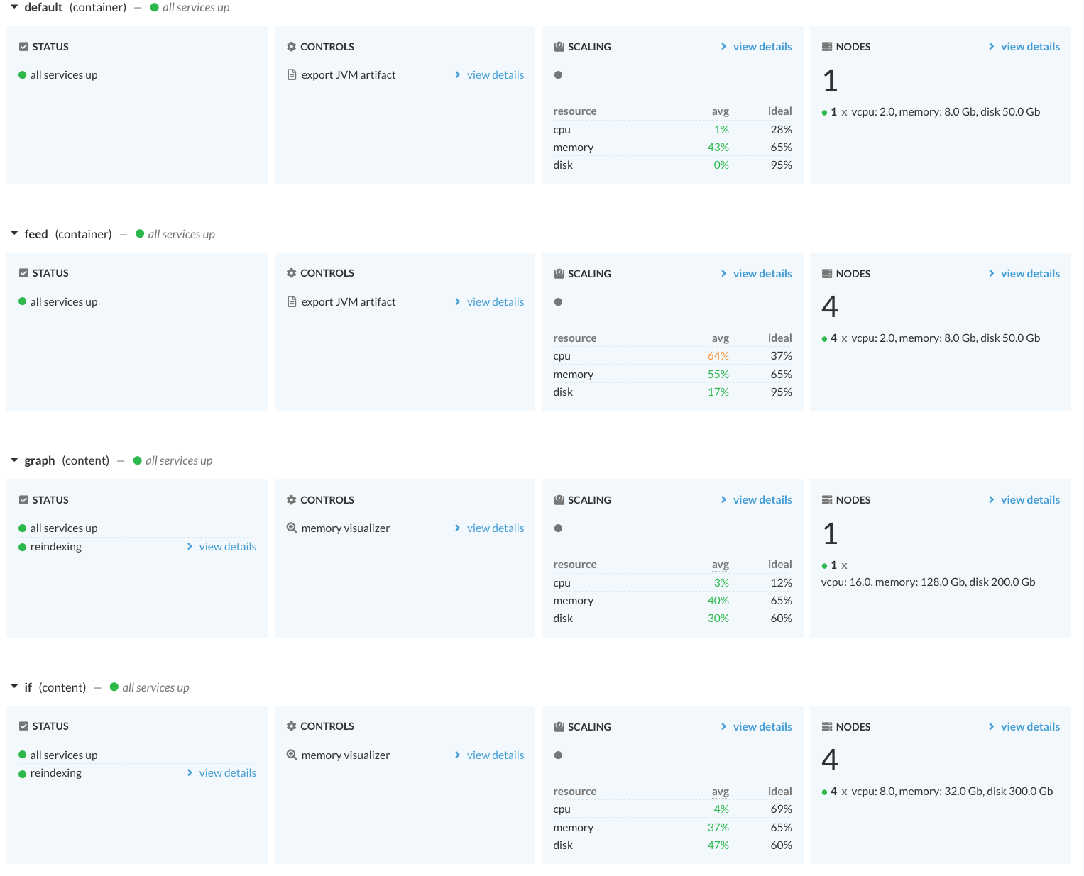Screenshot from Vespa Cloud console with app’s clusters and allocated resources.

As can be seen from the cluster resource scaling summary, the deployment is slightly over-provisioned and could support larger vector volumes comfortably. Vespa Cloud also allows a wide range of resource combinations (memory, CPU, disk) and the number of nodes per Vespa cluster.

Vespa stateless function components

Custom stateless Vespa functions implement the serving and processing logic. The components are deployed inside the Vespa cluster, where communication is secured, and data transferred with optimized binary protocols. The gist of the custom searcher implementing the search logic is given below:

@Override
public Result search(Query query, Execution execution) {
    Tensor queryVector = query.getTensor("query(q)");
    CentroidResult centroidResult = clustering.getCentroids(
        queryVector,
        nClusters,
        hnswExploreHits,
        execution);
    List<Centroid> centroids = clustering.prune(
        centroidResult.getCentroids(),
        pruneThreshold);

    DotProductItem dp = new DotProductItem("neighbors");
    for (Centroid c : centroids) {
        dp.addToken(c.getId(), c.getIntCloseness());
    }
    query.getModel().getQueryTree().setRoot(dp);
    query.getModel().setSources("if");
    query.getRanking().setRerankCount(reRankCount);
    return mergeResult(execution.search(query), centroidResult);
}

See the full version.

Similarly, a custom document processor implements the search in the HNSW graph, and annotates the incoming vector with the nearest centroids. See AssignNeighborsDocProc.

Vespa HNSW-IF Experiments

The following experiments use these fixed indexing side hyperparameters:

• In-memory centroid indexing using the following HNSW settings: max-links-per-node: 18 and neighbors-to-explore-at-insert: 100.
• For any given non-centroid vector, the 12 closest centroid vector ids are indexed using the inverted index.

Batch indexing performance

With the mentioned allocated resources in Vespa Cloud perf, indexing the SPACEV-1B dataset takes approximately 28 hours. The 200M centroid vectors are fed first and indexed at around 9000 puts/s into the HNSW graph content cluster. The remaining 800M non-centroid vectors are indexed with similar puts/s, and also search the HNSW index at the same rate.

Vectors are read from the dataset and converted to Vespa JSON feed format by a python script. The resulting two JSON files are fed using Vespa feed client for ultimate batch feed performance using http/2 with mTls to secure the vector data in transit. Vespa Cloud also stores all data using encryption (encryption at rest).

Vespa Cloud console screenshot, taken during indexing of non-centroid vectors.

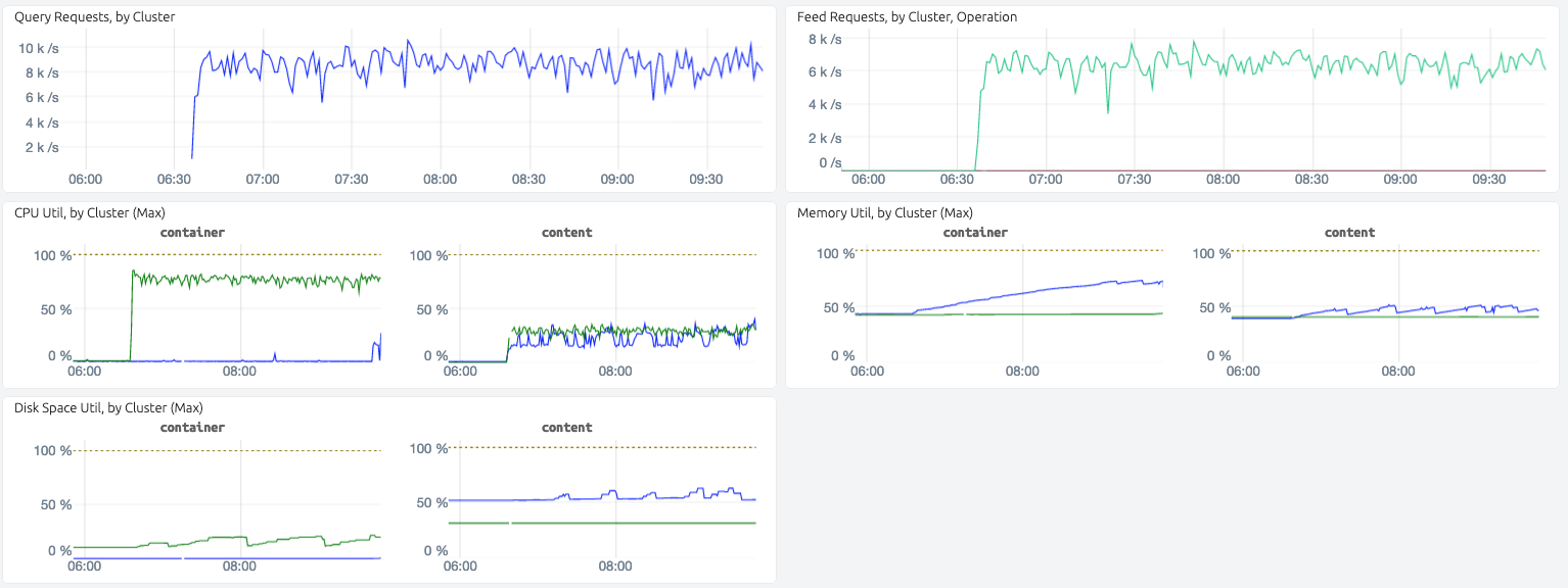Vespa Cloud metrics dashboard.

The Vespa Cloud metrics provide insight into resource utilization which can help choose the right instance resource specification.

HNSW-IF accuracy

Any approximate vector search use case needs to quantify the accuracy impact of using approximate search instead of exact search. Using the ground truth neighbors for the 29,3K SPACEV-1B query vectors, we can quantify recall@10 with the hybrid HNSW-IF solution:

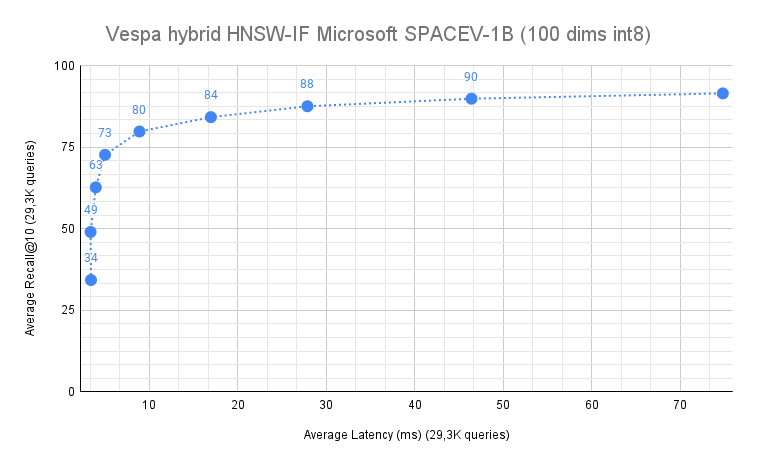Recall@10 for 29,3K queries

The above figure is produced by running all 29,3K queries with an increasing number of k centroids, ranging from 1 centroid to 256 centroids (1, 2, 4, 8 , 16, 32, 64, 128, 256). The distance prune threshold was set to 0.6, and the maximum re-ranking depth was 4K. Example run using recall.py with 32 centroid clusters k=32, re-ranking at most 4K vectors.

$ python3 recall.py --endpoint https://spann.samples.aws-us-east-1c.perf.z.vespa-app.cloud/search/ \
  --query_file query.i8bin \
  --query_gt_file public_query_gt100.bin \
  --clusters 32 \
  --distance_prune_threshold 0.6 \
  --rank_count 4000 \
  --certificate data-plane-public-cert.pem \
  --key data-plane-private-key.pem

With k=128 centroids, we reach 90% recall@10 at just below 50 ms end-to-end. 50 ms is one order of magnitude larger than what in-memory algorithms support at the same recall level, but for many vector search use cases, 50ms is perfectly acceptable, especially considering the high recall. To put the number in context, 9 out of 10 queries return the same top-10 result as the expensive nearest neighbor search, over 1B vectors!

Summary

This blog post introduced a cost-effective hybrid method for billion-scale vector search, enabling many new real-world applications using AI-powered vector representations. Today, You can get started using the ready-to-deploy billion-scale-vector-search.

Also try other Vespa sample applications built using Vespa’s approximate nearest neighbor search support using HNSW:

• State-of-the-art text ranking: Vector search with AI-powered representations built on NLP Transformer models for candidate retrieval. The application has multi-vector representations for re-ranking, using Vespa’s phased retrieval and ranking pipelines. Furthermore, the application shows how embedding models, which map the text data to vector representation, can be deployed to Vespa for run-time inference during document and query processing.

• State-of-the-art image search: AI-powered multi-modal vector representations to retrieve images for a text query.

These are examples of applications built using AI-powered vector representations and where real-world deployments need query-time constrained nearest neighbor search.

Vespa is available as a cloud service; see Vespa Cloud - getting started, or self-serve Vespa - getting started.