Photo by Vincentiu Solomon on Unsplash

In the first post in this series, we introduced compact binary-coded vector representations that can reduce the storage and computational complexity of both exact and approximate nearest neighbor search. This second post covers an experiment using a 1-billion binary-coded representation derived from a vector dataset used in the big-ann-benchmark challenge. The purpose of this post is to highlight some of the trade-offs related to approximate nearest neighbor search, and especially we focus on serving performance versus accuracy.

Vespa implements a version of the HNSW (Hierarchical Navigable Small Word) algorithm for approximate vector search. Before diving into this post, we recommend reading the HNSW in Vespa blog post explaining why we chose the HNSW algorithm.

Choosing a Vector Dataset

When evaluating approximate nearest neighbor search algorithms it is important to use realistic vector data. If you don’t have the vectors for your problem at hand, use a publicly available dataset.

For our experiments, we chose the Microsoft SPACEV-1B from Bing as our base vector dataset.

This is a dataset released by Microsoft from SpaceV, Bing web vector search scenario, for large scale vector search-related research usage. It consists of more than one billion document vectors and 29K+ query vectors encoded by the Microsoft SpaceV Superior model.

The vector dataset was published last year as part of the big-ann-benchmarks (https://big-ann-benchmarks.com/) challenge. It consists of one billion 100-dimensional vectors using int8 precision. In other words, each of the hundred vector dimensions is a number in the [-128,127] range. The dataset has 29,3K queries with pre-computed ground truth nearest neighbors using the euclidean distance for each query vector. Vespa supports four different tensor vector precision types, in order of increasing precision:

• int8 (8 bits, 1 byte) per dimension
• bfloat16 (16 bits, 2 bytes) per dimension
• float (32 bits, 4 bytes) per dimension
• double (64 bits, 8 bytes) per dimension

Quantization and dimension reduction as part of the representation learning could save both memory and CPU cycles in the serving phase, and Microsoft researchers have undoubtedly had this in mind when using 100 dimensions with int8 precision for the embedding.

In the first post in this series we discussed some of the benefits of working with binarized vector datasets where the original vector representation (e.g, int8) is transformed to binary. We don’t train a binary representation model, but instead use the unsupervised sign threshold function. Using the threshold function, we convert the mentioned SPACEV-1B vector dataset to a new and binarized dataset. Both queries and document vectors are binarized, and we use the hamming distance metric for the nearest neighbor search (NNS) with our new dataset.

import numpy as np
import binascii
#vector is np.array([-12,3,4....100],dtype=np.int8)
binary_code = np.packbits(np.where(vector > 0, 1,0)).astype(np.int8)

_{Binarization using NumPy}

The binarization step packs the original vector into 104 bits, which is represented using a 13 dimensional dense single-order int8 tensor in Vespa.

However, this transformation from euclidean to hamming does not preserve the original euclidean distance ordering, so we calculate a new set of ground truth nearest neighbors for the query dataset using hamming distance. Effectively, we create a new binarized vector dataset which we can use to experiment and demonstrate some trade-offs related to vector search:

• Brute force nearest neighbor search using multiple search threads to parallelize the search for exact nearest neighbors
• Approximate nearest neighbor search where we accept an accuracy loss compared to exact search.
• Indexing throughput with and without HNSW enabled
• Memory and resource utilization with and without HNSW enabled

As described in the first post in this series, we can also use the hamming distance as the coarse level nearest neighbor search distance metric and re-rank close vectors in hamming space using the original representation’s euclidean distance. In our experiments, we focus on the new binarized dataset using hamming distance.

Experimental setup

We deploy the Vespa application to the Vespa cloud performance zone, and use the following node resources for the core Vespa service types, see services.xml reference guide for details:

2x Stateless container with search API (<search>)

<nodes count="2">
  <resources memory="12Gb" vcpu="16" disk="100Gb"/>
</nodes>

2x Stateless container with feed API (<document-api>)

<nodes count="2">
  <resources memory="12Gb" vcpu="16" disk="100Gb"/>
</nodes>

1x Stateful content cluster with one node for storing and indexing the vector dataset

<nodes count="1">
  <resources memory="256Gb" vcpu="72" disk="1000Gb" disk-speed="fast"/>
</nodes>

This deployment specification isolates resources used for feed and search, except for search and indexing related resource usage on the content node. Isolating feed and search allows for easier on-demand resource scaling as the stateless containers can be auto-scaled faster with read and write volume than stateful content resources. For self-hosted deployments of Vespa, you need to list the nodes you are using, and there is no auto-scaling.

The following is the base Vespa document schema we use throughout our experiments:

schema code {
  document code {
    field id type int {
      indexing: summary|attribute
    }
    field binary_code type tensor<int8>(b[13]) {
      indexing: attribute
      attribute {
        distance-metric:hamming
      }
    }
  }
}

_{Vespa document schema without HNSW indexing enabled}

Evaluation Metrics

To evaluate the accuracy degradation when using approximate nearest neighbor search (ANNS) versus the exact ground truth (NNS), we use the Recall@k metric, also called Overlap@k. Recall@k measures the overlap between the k ground truth nearest neighbors for a query with the k nearest returned by the approximate search.

The evaluation routine handles distance ties; if a vector returned by the approximate search at position k has the same distance as the ground truth vector at position k, it is still considered a valid kth nearest neighbor. For our experiments, we use k equal to 10. The overall Recall@10 associated with a given parameter configuration is the mean recall@10 of all 29,3K queries in the dataset.

Note that the vector overlap metric used does not necessarily directly correlate with application-specific recall metrics. For example, recall is also used in Information Retrieval (IR) relevancy evaluations to measure if the judged relevant document(s) are in the retrieved top k result. Generally, degrading vector search Recall@k impacts the application-specific recall, but much depends on the use case.

For example, consider the Efficient Passage Retrieval with Hashing for Open-domain Question Answering paper discussed in the previous post in this series. The authors present a recall@k metric for k equal to 1, 20 and 100. This specific recall@k measures if the ground truth golden answer to the question is in any top k retrieved passage. In this case, the error introduced by using approximate search might not impact the use case recall@k metric since the exact answer to the question might exist in several retrieved documents. In other words, not recalling a record with the ground truth answer due to inaccuracy introduced by using approximate vector search does not necessarily severely impact the end-to-end recall metric.

Similarly, when using ANNS for image search at a web scale, there might be many equally relevant images for almost any query. Therefore, losing relevant “redundant” pictures due to nearest neighbor search accuracy degradation might not impact end-to-end metrics like revenue and user satisfaction severely.

However, reducing vector recall quality will impact other applications using nearest neighbor search algorithms. Consider, for example, a biometric fingerprint recognition application that uses nearest neighbor search to find the closest neighbor for a given query fingerprint in a database of many fingerprints. Accepting any accuracy loss as measured by Recall@1 (the true closest neighbor) will have severe consequences for the overall usefulness of the application.

Vector Indexing performance

We want to quantify the impact of adding data structures for faster and approximate vector search on vector indexing throughput. We use the Vespa HTTP feeding client to feed vector data to the Vespa instance.

Writing becomes more expensive when enabling HNSW indexing for approximate vector search. This is because insertion into the HNSW graph requires distance calculations and graph modifications which reduces overall throughput. Vespa’s HNSW implementation uses multiple threads for distance calculations during indexing, but only a single writer thread can mutate the HNSW graph. The single writer thread limits concurrency and resource consumption. Generally, Vespa balances CPU resources used for indexing versus searching using the concurrency setting.

Vespa exposes two core HNSW construction parameters that impacts feeding performance (and quality as we will see in subsequent sections):

• max-links-per-node Specifies how many links are created per vector inserted into the graph. The default value in Vespa is 16. The HNSW paper calls this parameter M.
  A higher value of max-links-per node increases memory usage and reduces indexing throughput, but also improves the quality of the graph.

• neighbors-to-explore-at-insert Specifies how many neighbors to explore when inserting a vector in the HNSW graph. The default value in Vespa is 200. This parameter is called efConstruction in the HNSW paper. A higher value generally improves the quality but lowers indexing throughput as each insertion requires more distance computations. This parameter does not impact memory footprint.

We experiment with the following HNSW parameter combinations for evaluating feed indexing throughput impact.

• No HNSW indexing for exact search
• HNSW with max-links-per-node = 8, neighbors-to-explore-at-insert 48
• HNSW with max-links-per-node = 16, neighbors-to-explore-at-insert 96

The document schema, with HNSW indexing enabled for the binary_code field looks like this for the last listed parameter combination:

schema code {
  document code {
    field id type int {
      indexing: summary|attribute
    }
    field binary_code type tensor<int8>(b[13]) {
      indexing: attribute|index
      attribute {
        distance-metric:hamming
      }
      index {
        hnsw {
          max-links-per-node: 16
          neighbors-to-explore-at-insert: 96
        }
      }
    }
  }
}

_{Vespa document schema with HNSW enabled}

The real-time indexing throughput results are summarized in the following chart:

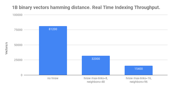
_{Real-time indexing performance without HNSW indexing and with two HNSW parameter combinations.}

Without HNSW enabled, Vespa is able to sustain 80 000 vector puts/s. By increasing the number of nodes in the Vespa content cluster using Vespa’s content distribution, it is possible to increase throughput horizontally. For example, using four nodes instead of one, would support 4x80 000 = 320 000 puts/.

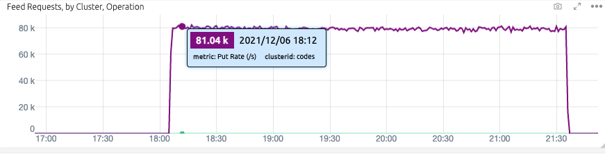
_{Sustained real-time indexing without HNSW, screenshot from Vespa Cloud Metrics}

When we introduce HNSW indexing, the write-throughput drops significantly as it involves mutations of the HNSW graph and distance calculations. In addition to indexing throughput, we also measure peak memory usage for the content node:

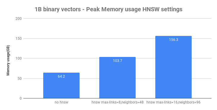
_{Peak Memory Usage without HNSW indexing and with two HNSW parameter combinations.}

Now, you might ask, why are Vespa using 64G of memory for this dataset in the baseline case without HNSW?
The reason is that Vespa stores the global document id (a 96-bit hash of the document id string) in memory, and the document id consumes more memory than the vector data alone. One billion document identifiers consume about 33GB of memory. Finally, there is also 4GB of data for the integer id attribute. This additional memory used for the in-memory gid, is used to support fast elastic content distribution, fast partial updates and more.

As we introduce HNSW indexing, the memory usage increases significantly due to the additional HNSW graph data structure which is also in memory for fast access during searches and insertions.

Brute-force exact nearest neighbor search performance

As we have seen in the indexing performance and memory utilization experiments, not using HNSW uses considerably less memory, and is the clear indexing throughput winner - but what about the search performance of brute force search? Without HNSW graph indexing, the complexity of the search for neighbors is linear with the total document volume, so that is surely slow for 1B documents?

To overcome the latency issue, we can use one of the essential Vespa features: Executing a query using multiple search threads. By using more threads per query, Vespa can make better use of multi-CPU core architectures and reduce query latency at the cost of increased CPU usage per query. See more on scaling latency versus throughput using multithreaded search in the Vespa sizing and performance guide.

To easily test multiple threading configurations, we deploy multiple Vespa rank profiles. Choosing ranking profile is done in the query, so it’s easy to run experiments without having to re-deploy the application.

rank-profile hamming {
  num-threads-per-search:1
  first-phase {
    expression:closeness(field,binary_code)
  }
}

rank-profile hamming-t2 inherits hamming {
  num-threads-per-search:2
}
..

_{Ranking profiles defined in the document schema.}

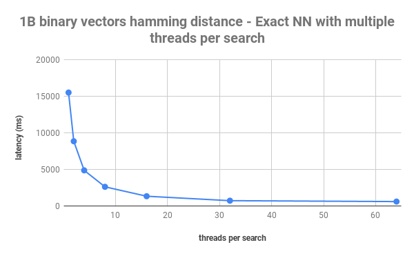
_{Exact nearest neighbor search performance versus threads used per query.}

As we can see from the figure above, one search thread uses on average 15 seconds to compute the exact nearest neighbors. By increasing the number of search threads per query to 32, we can reach sub-second search latency. The catch is that at as low as one query per second (QPS), the node would be running at close to 100% CPU utilization. Still, trading latency over throughput might be a good decision for some use cases that do not require high query throughput or where CPU utilization is low (over-provisioned resources). In our case, using all available CPU cores for our exact ground truth calculations reduced the overall time duration significantly.

Approximate nearest neighbor search performance

Moving from exact to approximate nearest neighbor search, we evaluate the search performance versus accuracy using the recall@10 metric for the same HNSW parameter combinations we used to evaluate indexing performance:

• max-links-per-node = 8, neighbors-to-explore-at-insert 48
• max-links-per-node = 16, neighbors-to-explore-at-insert 96

We use the exact search to obtain the 100 ground truth exact nearest neighbors for all the queries in the dataset, and use those for the approximate nearest neighbor search recall@10 evaluation. We use 100 in the ground truth set to be able to take into account distance ties.

With approximate nearest neighbor search in Vespa, the traversal of the HNSW graph uses one thread per search irrespective of the number of configured rank profile search threads; the threads are put to use if the ranking profile uses higher-level subsequent ranking phases. For use cases and ranking profiles without higher level ranking phases, we recommend explicitly configuring one thread to avoid idling searcher threads which are not used for the graph traversal. Recall@10 versus latency is provided in the figure below:

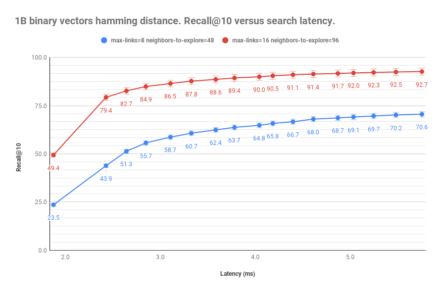
_{Approximate nearest neighbor search performance versus recall@10.}

We produce the graph by running all 29,3K queries in the binarized dataset and computing the recall@10 and measure the latency for different run time values of hnsw.exploreAdditionalHits. The hnsw.exploreAdditionalHits run-time parameter allows us to tune quality versus cost without re-building the HNSW graph.

As we can see from the above graph, using more indexing resources with more links and more distance calculations during graph insertion improves the search quality at the same cost/latency. As a result, we reach 90% recall@10 instead of 64% recall@10 at the exact cost of 4 ms search time. Of course, the level of acceptable recall@10 will be use case dependent, but the above figure illustrates the impact on search quality when using different construction HNSW parameters.

Furthermore, comparing the 4ms at 90% recall@10 with the exact nearest neighbor search performance of 15000 ms, we see that we achieve a speedup of 3,750x. Note that these are latency numbers for single-threaded searches. For example, with 4 ms average latency per search using one thread, a node with one CPU core will be able to evaluate up to about 250 queries per second. 72 CPU cores would be 72x that, reaching 18,000 queries per second at 100% CPU utilization. Scaling further for increased query throughput is achieved using multiple replicas using grouped content distribution (or more CPU cores per node). See more on how to size Vespa search deployments in the Vespa sizing guide.

Summary

In this blog post, we explored several trade-offs related to vector search.
We concluded that the quality, as measured by recall@k, must be weighed against the use case metrics and the deployment cost. Furthermore, we demonstrated how multithreaded search could reduce the latency of the exact search, but scaling query throughput for exact search would be prohibitively expensive at this scale. However, using brute force search could be a valid and cost-effective alternative for smaller data volumes with low query throughput, especially since the memory usage is considerably less, and supported indexing throughput is higher.

In the next blog post in this series, we will experiment with the original Microsoft SPACEV-1B vector dataset, using the original dimension with int8 precision with euclidean distance. In the upcoming blog post we will explore a hybrid approach for approximate nearest neighbor search. This approach uses a combination of inverted indexes and HNSW, which reduces memory usage. The method we will explore using Vespa is highly inspired by the SPANN: Highly-efficient Billion-scale Approximate Nearest Neighbor Search paper. Stay tuned!