
Summary
Searching for the nearest neighbors of a data point in a high dimensional vector space is an important problem for many real-time applications. For example, in Computer Vision it can be used to find similar images in large image datasets. In Information Retrieval, pre-trained text embeddings can be used to match documents based on the distance between query and document embeddings. In many of these applications, the document corpus is constantly evolving and the search is constrained by query filters applied on the metadata of the data points. For example, in E-commerce, a nearest neighbor search for products in a vector space would typically be constrained by product metadata like inventory status and price.
Vespa (the open source big data serving engine) already supports exact nearest neighbor search that is integrated with the Vespa query tree and its filter support. This enables you to get the exact nearest neighbors meeting the filter criterias of the query. This works well when the number of documents to calculate nearest neighbors for is small, e.g when the query filter is strong, or the document corpus is small. However, as the number of documents to consider increases, we want to trade exactness for performance and we need an approximate solution.
This blog post is part 1 in a series of blog posts where we share how the Vespa team implemented an approximate nearest neighbor (ANN) search algorithm. In this first post, we’ll explain why we selected HNSW (Hierarchical Navigable Small World Graphs) as the baseline algorithm and how we extended it to meet the requirements for integration in Vespa. Requirements included supporting real-time updates, integration with the Vespa query tree, and being flexible enough to fit a wide range of use cases.
Requirements & Challenges
Vespa is an open source real-time big data serving engine. In a typical application, the document corpus is constantly evolving. New documents are added and removed, and metadata is being updated. A typical use case is news article search and recommendation, keeping a week, month or year’s worth of articles, continually adding or updating new articles while selectively removing the oldest ones. In this case, nearest neighbor search over pre-trained text embeddings could be used in combination with query filters over metadata.
Based on the existing functionality and flexibility of Vespa, we defined a set of requirements an ANN search algorithm had to support to be a good fit for integration:
- Indexes used in the algorithm must be real-time updateable with low latency and high throughput. Data points can be added, updated and removed, and the entire corpus should not be needed when creating the index.
- Concurrent querying with low latency and high throughput without huge performance impact due to ongoing update operations.
- Seamless integration with the Vespa query tree and its filter support. This enables correct results, compared to just increasing top K for the nearest neighbor search algorithm to compensate when query filters are used.
Algorithms Background
There exists a lot of algorithms for ANN search. Many of these are summarized and analyzed in Approximate Nearest Neighbor Search on High Dimensional Data — Experiments, Analyses, and Improvement (v1.0) and A Revisit of Hashing Algorithms for Approximate Nearest Neighbor Search. In addition, benchmark results for different algorithms over different datasets are summarized in ANN Benchmarks.
Existing algorithms are mainly focused on a stable document corpus where all data points in the vector space are known up front. In this case the index structure is built once, and then used for nearest neighbor searches. To support real-time updates, we looked for algorithms that were either incremental in nature or could be modified to meet this requirement.
There are three broad categories of algorithms: tree-based, graph-based and hash-based. We choose one from each category for a more detailed exploration. This selection was based on how they performed in benchmarks within papers and in ANN Benchmarks, and how easy the algorithm was to modify to fit our requirements.
We ended up with the following:
- Annoy
Annoy is tree-based and described in Nearest neighbors and vector models – part 2 – algorithms and data structures. It takes a straightforward engineering approach to the ANN problem, and is quite easy to understand and implement. An Annoy index consists of N binary trees, where each tree partitions the vector space using random hyperplanes at each node in the tree. The implementation is available on github. - HNSW - Hierarchical Navigable Small World Graphs
This is graph-based and described in Efficient and robust approximate nearest neighbor search using Hierarchical Navigable Small World graphs. HNSW builds a hierarchical graph incrementally, and has great search performance with high recall, motivating us to prototype it for comparison. Each node in the graph represents a point in the vector space, and nodes are linked to other nodes that are close in space. The implementation is available on github. - RPLSH - Random Projection based Locality Sensitive Hashing
This is hash-based and described in A Revisit of Hashing Algorithms for Approximate Nearest Neighbor Search. The implementation is available on github. Since the random hyperplanes used for projections can be selected up-front (only depending on the number of dimensions of the vector space) this approach is data-independent. For our purposes, we could use the hash value as a filter, where only documents having most bits in common with the hash value of the query data point would be considered for full distance computation. This would give us little extra memory and CPU usage and would be easy to fit into our exact (brute-force) nearest neighbor feature. It was the first algorithm that we implemented as a prototype. However, in our prototype we found that getting a significant speedup required a large sacrifice of quality. For more info, see Dropping RPLSH below.
We created prototype implementations of the three algorithms in C++. This gave us a deeper understanding and the ability to make necessary modifications to support real-time updates and query filters. The prototypes were also used to do low-level benchmarking and quality testing.
Prototype Benchmark
We benchmarked the three prototype implementations to look at indexing throughput and search throughput with different document corpus sizes. We used the 1M SIFT (128 dim) and 1M GIST (960 dim) datasets, where one vector corresponds to a document. In this section, we summarize the results of the 1M SIFT tests. Findings were similar with the 1M GIST dataset.
Setup
The tests were executed in a CentOS 7 Docker image using Docker Desktop on a MacBook Pro (15 inch, 2018) with a 2.6 GHz 6-Core Intel Core i7 CPU and 32GB of memory. The Docker setup was 8 CPUs, 16GB of memory and 1GB of Swap.
The configuration of the algorithms were as follows:
- Float size: 4 bytes.
- Annoy: Number of trees = 50. Max points in leaf node = 128.
- HNSW: Max links per node (M) = 16. Note that level 0 has 32 links per node (2*M). Number of neighbors to explore at insert (efConstruction) = 200.
- RPLSH: 512 bits used for hash and linear scan of hash table.
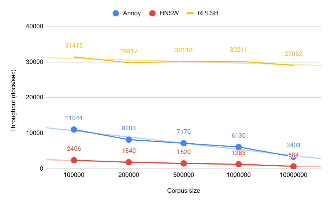
Indexing Throughput
The 1M SIFT dataset was split into chunks of first 100k, 200k, and 500k vectors, and indexing throughput was tested with different corpus sizes. The index structures for all algorithms started empty, and we added one document at a time to simulate real-time feeding. One thread was used. Necessary adjustments to the prototype implementations were done to accommodate this. Note that the data points for 10M documents are estimated based on the 100k and 1M data points.
Observations:
- Indexing throughput depends on corpus size for Annoy and HNSW, where throughput is halved when corpus size is increased by 10x.
- Indexing throughput for RPLSH is independent of corpus size.
- Annoy is 4.5 to 5 times faster than HNSW.
- RPLSH is 23 to 24 times faster than HNSW at 1M documents.
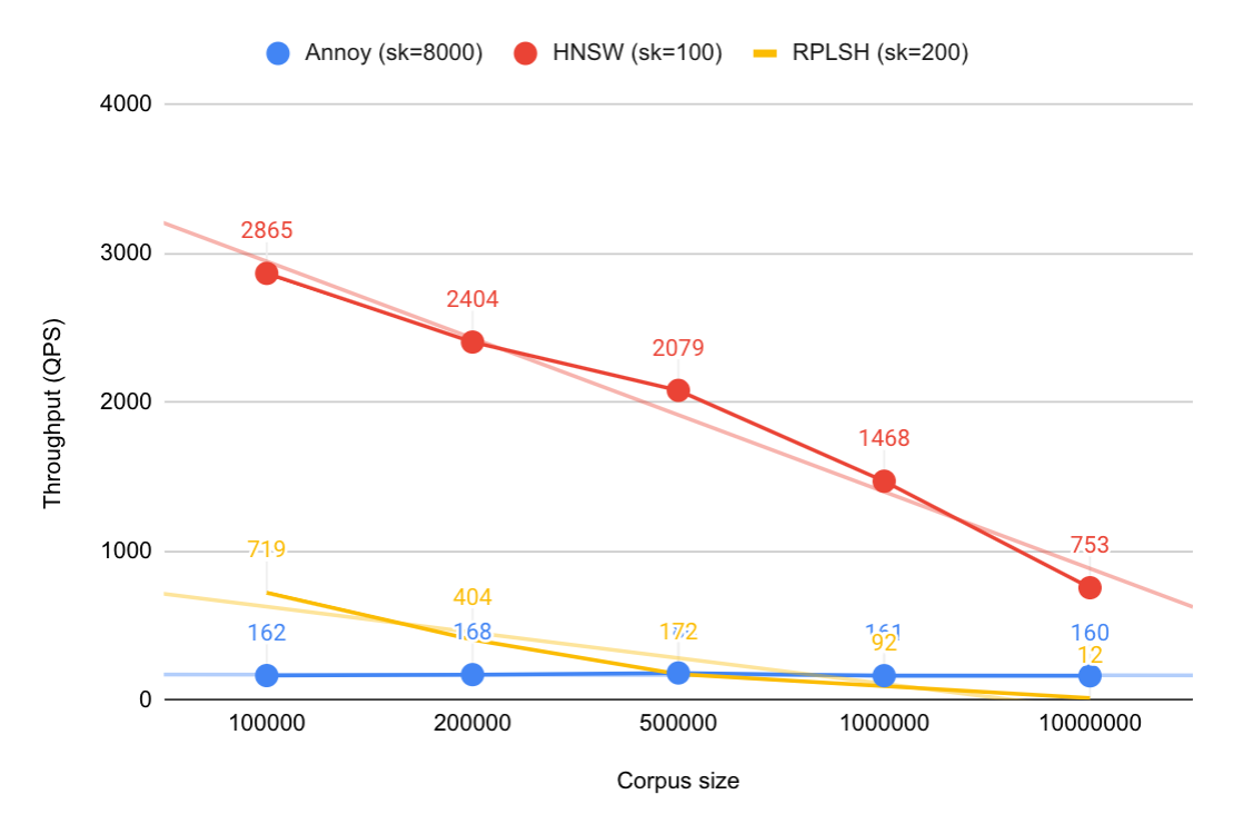
Search Throughput (QPS)
The search throughput was measured after the indexes were built, using a single benchmarking client and search thread. We used the query vectors from the dataset, and searched for the nearest K=100 neighbors from the query vector. To get comparable quality results between the algorithms we had to adjust some of the parameters used. The default behavior for Annoy is to collect K=100 candidates per tree, and then calculate brute force distance for all those. To get comparable quality between Annoy and HNSW we had to collect 8000 candidates instead of 5000. For RPLSH, we used the Hamming distance between hashes to pre-filter candidates after collecting 200 candidates into a heap, skipping full distance calculation for most candidates. For HNSW, we asked for 100 candidates.
Observations:
- HNSW outperforms Annoy and RPLSH. At corpus size 1M the QPS is 9 times as high as Annoy, and 16 times as high as RPLSH at comparable quality. Similar observations between hnswlib and Annoy are found in ANN Benchmarks, where the QPS of hnswlib is 5-10 times higher at the same quality on all tested datasets.
- The HNSW search algorithm depends heavily on the number of links between nodes, which again depends on corpus size. The QPS is halved when the corpus size is increased by 10x. We see the same during indexing as that uses the search algorithm to find candidates to connect to.
- The Annoy search algorithm is less dependent on corpus size, at least with small corpus sizes. The static cost is driven by brute force calculation of distances for the candidate set, 8000 in this case. With high corpus size the cost of traversing the binary trees will likely match and exceed the static cost. We don’t know where this limit is.
- For RPLSH, doing exhaustive search (linear scan) of the hashes is more expensive than expected. One major consideration here is that the data reduction (from 128 dimensions*32 bit floats, to 512 bits hash) is just a factor 8, and indeed we got around 8 times speedup compared to brute-force linear scan.
Index Structures & Memory Usage
The prototype implementations used simple data structures to represent the index structures of the algorithms in memory. Only one thread was used for indexing and searching and we didn’t have to worry about locking. These challenges would have to be overcome in the actual implementation of the selected algorithm. We created a rough index structure design for both Annoy and HNSW to see how much memory the index would use.
In Vespa, a data point in a high dimensional vector space is represented by a tensor of rank one with dimension size equal to the dimensionality of the vector space. To use this, a document type with a tensor field of such type is defined, and documents with tensors are fed to Vespa. A document type typically consists of multiple other fields as well, for instance, metadata fields and other tensor fields. The tensors across all documents for a given tensor field are stored in-memory. The index structures were designed such that they just reference the tensor data points stored in-memory. In addition, they support one writer thread doing changes, while multiple reader threads are searching, without use of locking. The actual index structure details for HNSW will be covered in an upcoming blog post.
Annoy Index
An Annoy index consists of multiple binary trees. Each tree consists of split nodes and leaf nodes. A split node has an offset from origo, a hyperplane that splits the space in two, and reference to left and right child nodes. A leaf node contains the document ids of the points that ended up in that portion of space. The document ids are used to lookup the actual tensor data from memory.
HNSW Index
An HNSW index consists of navigable small world graphs in a hierarchy. Each document in the index is represented by a single graph node. Each node has an array of levels, from level 0 to n. The number of levels is constant during the lifetime of the node and is drawn randomly when the node is created. All nodes have at least level 0. At each level there is a link array which contains the document ids of the nodes it is connected to at that level. The document ids are used to lookup the actual tensor data points from memory.
Memory Usage Summary
The following summarizes the memory usage of the Annoy and HNSW indexes over the 1M SIFT dataset. The configuration is the same as used on the prototypes when benchmarking indexing and search. The memory usage for storing the hash values in RPLSH, 512 bits per document, is also shown for reference.
Observations:
- The Annoy index is almost 3 times larger than the HNSW index, which results in ~40% more total memory usage in the 1M SIFT dataset.
- Both indexes are independent of dimension size, but max points in a leaf node (Annoy) and max links per level (HNSW) might need adjustments with higher dimensionality to get decent quality.
| Annoy index | HNSW index | RPLSH hash | |
|---|---|---|---|
| Total tensor size (MB) | 488 | 488 | 488 |
| Total index size (MB) | 387 | 134 | 61 |
| Total size (MB) | 875 | 622 | 549 |
| Index percent of total | 44% | 22% | 11% |
Dropping RPLSH
To get good quality (recall) with RPLSH we found that a large hash size was needed. Running a quality benchmark on the SIFT dataset with 1M data points, shows the recall (as percentage of correct hits when asking for top K=100) is bad with a 64 bit hash. You would need to do a full distance calculation for 25000 documents just to get 80% recall. We worked mostly with a 512-bit hash, where (on average) you should get 80% recall with just 600 candidates, and 90% recall with 1200 candidates.
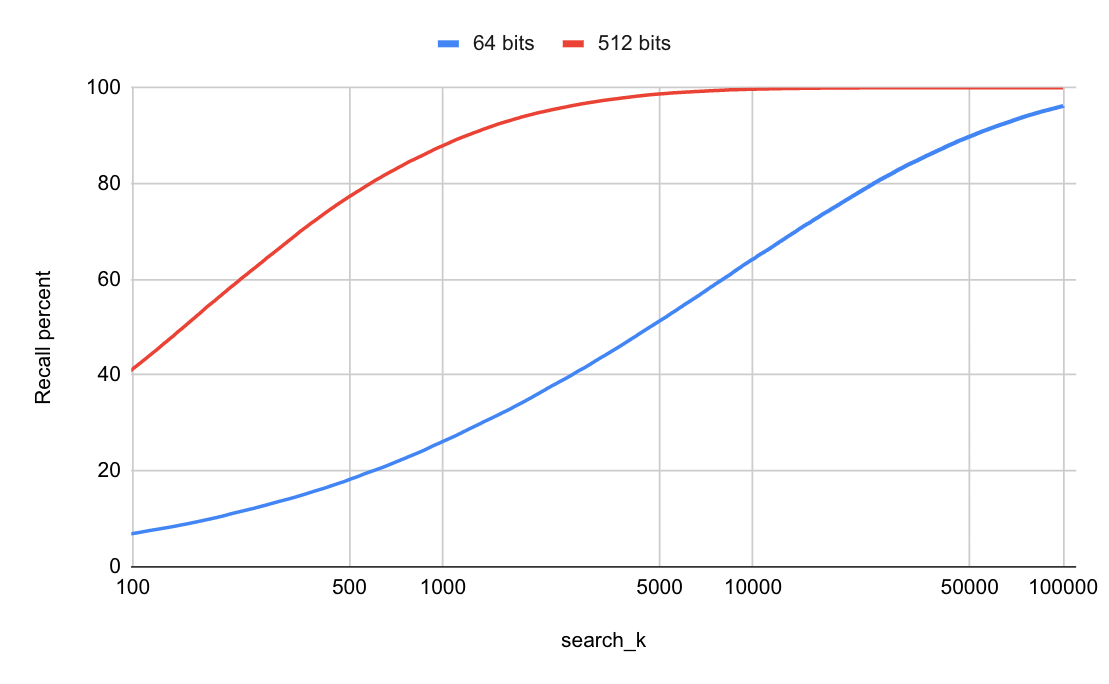
With 512-bit hashes, doing a linear scan of the table of hash values doesn’t scale well, and some sort of index structure to search in the transformed space is necessary.
Choosing HNSW
Several factors were considered when choosing HNSW as the algorithm to use as a baseline for integration in Vespa. We needed an algorithm with good performance and low resource usage, that was possible to extend and integrate in Vespa.
As seen in the previous section, none of the algorithms have both good indexing and search performance. We needed to make tradeoffs. As stated in the introduction, an approximate algorithm is needed to improve the search performance compared to the exact algorithm already supported in Vespa. Based on this criteria alone, HNSW is the clear winner. Indexing performance is worse, but this is a tradeoff worth taking for the most common Vespa use cases. This is the reason indexing is done in the first place, to prepare data structures such that search is fast. Also, the index structure for HNSW uses significantly less memory than Annoy.
HNSW is also a good fit when it comes to the simplicity of integration in Vespa. Building the index is inherently incremental, so adding new data points in real-time is already handled. The Annoy algorithm must be changed to get similar functionality, as it uses all data points when drawing the random hyperplane splits. Removing data points is also handled in HNSW by having a “deleted” flag on each data point, but this is not a solution that will work well in Vespa. Datasets typically evolve over a long period of time, and the size of the index would just keep on growing, dominated by deleted points. We addressed this with an explicit remove strategy that removes nodes from the graph while re-linking the neighbors. The details will be described in the next blog post.
The last requirement for the chosen algorithm is that it works well with query filters. We experimented with a 2-phase solution for both the HNSW and Annoy prototypes. First, only the query filter is evaluated, resulting in the set of document ids passing the filter. Then this set is used in the search algorithm to only select neighbors that passed the filter. This is a simple and effective solution that works well when the amount of documents that are filtered away is not too high.
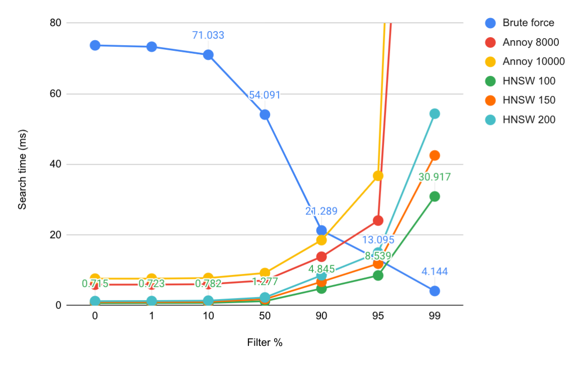
Exact vs Approximate
In prototype testing with the 1M SIFT dataset we observed that when more than 90-95% of the documents were filtered away, calculating the exact nearest neighbors after filtering was cheaper than searching the HNSW index with the filter discarding candidate hits. This is illustrated in the graph below.
Conclusion
In this blog post, we explored how the Vespa team selected HNSW (Hierarchical Navigable Small World Graphs) as the baseline approximate nearest neighbor algorithm for integration in Vespa. We needed an algorithm that could be extended to support real-time updates and work together with query filters. Benchmarking showed that HNSW has superior search performance and uses significantly less memory than Annoy. Building of the index is also inherently incremental. In addition we created a strategy for supporting proper removes.
In the next blog post, we will look at the actual index structure details for HNSW and how we implemented and integrated it in Vespa.