Photo by Federico Beccari on Unsplash

NASA estimates that the Milky Way galaxy contains between 100 to 400 billion stars. A mind-blowing large number of stars and solar systems, and also a stunning sight from planet earth on a clear night.

Many organizations face challenges involving star-sized datasets, even orders of magnitude larger. AI-powered representations of unstructured data like image, text, and video have enabled search applications we could not foresee just a few years ago. For example, in a previous blog post, we covered vision and video search applications using AI-powered vector representations.

Searching star-sized vector datasets using (approximate) nearest neighbor search is a fascinating and complex problem with many trade-offs :

• Accuracy of the approximate versus the exact nearest neighbor search
• Latency and scaling
• Scaling search volume (searches per second)
• Batch indexing versus real-time indexing and handling of updates and vector meta-data
• Distributed search in large vector datasets which does not fit into a single content node
• Cost($), total cost of ownership, including development efforts

This blog series looks at how to represent and search billion-scale vector datasets using Vespa, and we cover many of the mentioned trade-offs.

In this first post we look at compact binary-coded vector representations which can reduce storage and computational complexity of both exact and approximate nearest neighbor search. For those that are new to Vespa we can recommend reading the Vespa overview and the Vespa quick start guide before diving into this post.

Introduction

Deep Neural Hashing is a catchy phrase for using deep neural networks for learning compact hash-like binary-coded representations. The goal of representation learning, deep or not, is to transform any data into a suitable representation that retains the essential information needed to solve a particular task, for example, search or retrieval. Representation learning for retrieval usually involves supervised learning with labeled or pseudo-labeled data from user-item interactions.

Many successful text retrieval systems use supervised representation learning to transform text queries and documents into continuous high-dimensional real-valued vector representations. Query and document similarity, or relevancy, is reduced to a vector distance metric in the representational vector space. To efficiently retrieve from large collection of documents, one can turn to approximate nearest neighbor search algorithms instead of exact nearest neighbor search. See for example the
pre-trained transformer language models for search blog post for an introduction to state-of-the-art text retrieval using dense vector representations.

Recently, exciting research has demonstrated that it is possible to learn a compact hash-like binary code representation instead of a dense continuous vector representation without much accuracy loss. In Efficient Passage Retrieval with Hashing for Open-domain Question Answering, the authors describe using a hashing layer on top of the bi-encoder transformer architecture to train a binary coded representation of documents and queries instead of continuous real-valued representation.

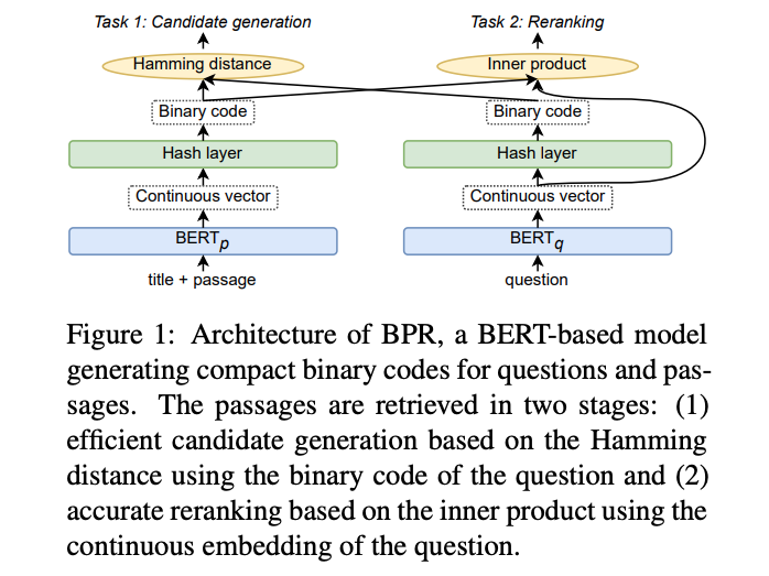
Illustration from Efficient Passage Retrieval with Hashing for Open-domain Question Answering

Note that the search is performed in two phases, first a coarse-level search using the hamming distance with binary codes, secondly a re-ranking phase using the continuous query vector representation and a unpacked vector representation from the binary code.

A huge advantage over continuous vector representations is that the binary-coded document representation significantly reduces the document storage requirements. For example, representing text documents in a 768-dimensional vector space where each dimension uses float precision, the storage requirement per document becomes 3072 bytes. Using a 768-bit binary-coded representation instead, the storage requirement per document becomes 96 bytes, a 32x reduction. In the mentioned paper, the authors demonstrate that the entire English Wikipedia consisting of 22M passages can be reduced to 2GB of binary codes.

Searching in binary-coded representations can be done using the hamming distance metric. The hamming distance between code q and code d is simply the number of bit positions that differ or, in other words, the number of bits that need to flip to convert q into d. Hamming distance is efficiently implemented on CPU architectures using few instructions (xor combined with population count). In addition, hamming distance search makes it possible to rank a set of binary codes for a binary coded query compared to exact hash table lookup.

Compact binary-coded representations paired with hamming distance is also successfully used for large-scale vision search. See for example these papers:

• Deep Learning of Binary Hash Codes for Fast Image Retrieval (pdf).
• TransHash: Transformer-based Hamming Hashing for Efficient Image Retrieval (pdf).

Representing hash-like binary-codes in Vespa

Vespa has first-class citizen support for representing high dimensional dense vectors using the Vespa tensor field type. Dense vectors are represented as dense first-order tensors in Vespa. Tensor cell values in Vespa support four numeric precision types, in order of increasing precision:

• int8 (8 bits, 1 byte) per dimension
• bfloat16 (16 bits, 2 bytes) per dimension
• float (32 bits, 4 bytes) per dimension
• double (64 bits, 8 bytes) per dimension

All of which are signed data types. In addition, for dense first-order tensors (vectors), Vespa supports fast approximate nearest neighbor search using Vespa’s HNSW implementation. Furthermore, the nearest neighbor search operator in Vespa supports several distance metrics, including euclidean, angular, and bitwise hamming distance.

To represent binary-coded vectors in Vespa, one should use first-order tensors with the int8 tensor cell precision type. For example, to represent a 128-bit code using Vespa tensors, one can use a 16-dimensional dense (indexed) tensor using int8 value type (16*8 = 128 bits). The Vespa document schema below defines a numeric id field of type int, representing the vector document id in addition to the binary-coded vector using a dense first-order tensor. The b denotes the tensor dimension name, and finally, [16] denotes the dimensionality.

schema code {
  document code {
    field id type int {}
    field binary_code type tensor<int8>(b[16]) {
      indexing: attribute
      attribute { 
        distance-metric:hamming
      } 
    }
  }
}

Using big-endian ordering for the binary-coded representation, the most significant bits from the binary-code at position 0 to 7 inclusive are the first vector element at index 0, bits at position 8 to 15 inclusive in the second vector element, and so on. For example, the following snippet uses NumPy with python to demonstrate a way to create a binary-coded representation from a 128-dimensional real-valued vector representation by using an untrained thresholding function (sign function):

import numpy as np
import binascii
vector = np.random.normal(3,2.5, size=(128))
binary_code = np.packbits(np.where(vector > 0, 1,0)).astype(np.int8)
str(binascii.hexlify(binary_code),'utf-8')
'e7ffef5df3bcefffbfffff9fff77fdc7'

The above hexadecimal string representation can be fed to Vespa using the Vespa JSON feed format.

{
  "id": "id:bigann:code::834221",
  "fields": {
    "id": 834221,
    "binary_code": {
      "values": "e7ffef5df3bcefffbfffff9fff77fdc7"
    }
  } 
}

Indexing in Vespa is real-time and documents become searchable within single digit millisecond latency at high throughput. The JSON feed files can be indexed with high throughput using the Vespa feed client.

Dense first-order tensors can either be in memory all the time or paged in from secondary storage on-demand at query time, for example, during scoring and ranking phases in a multiphased retrieval and ranking pipeline. In any case, the data is persisted and stored for durability and data re-balancing.

Furthermore, supporting in-memory and paged dense first-order tensors enables storing the original vector representation in the document model at a relatively low cost (storage hierarchy economics). For example, the following document schema keeps the original float precision vector on disk using the paged tensor attribute option.

schema code {
  document code {
    field id type int {} 
    field binary_code type tensor<int8>(b[16]) {
      indexing: attribute
      attribute { 
        distance-metric: hamming 
      }
    }
    field vector type tensor<float>(r[128]) {
      indexing: attribute
      attribute: paged
    }
  }
}

Storing the original vector representation on disk using the paged attribute option enables phased retrieval and ranking close to the data. First, one can use the compact in-memory binary code for the coarse level search to efficiently find a limited number of candidates. Then, the pruned candidates from the coarse search can be re-scored and re-ranked using a more advanced scoring function using the original document and query representation. Once a document is retrieved and exposed to the ranking phases, one can also use more sophisticated scoring models, for example using Vespa’s support for evaluating ONNX models.

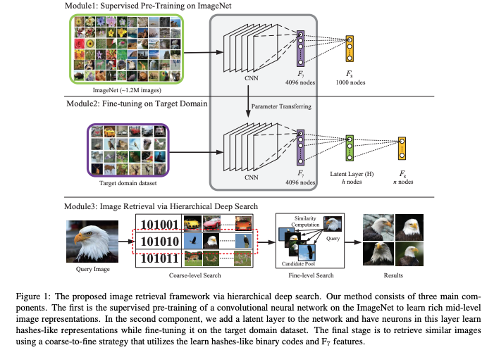
A two-phased coarse to fine level search using hamming distance as the coarse-level search.
Illustration from
Deep Learning of Binary Hash Codes for Fast Image Retrieval (pdf).

The binary-coded representation and the original vector are co-located on the same Vespa content node(s) since they live in the same document object. Thus, re-ranking or fine-level search using the real-valued vector representation does not require any network round trips to fetch the original vector representation from some external key-value storage system.

In addition, co-locating both the coarse and fine representation avoid data consistency and synchronizations issues between different data stores.

Searching binary-codes with Vespa’s nearest neighbor search query operator

Using Vespa’s nearest neighbor search query operator, one can search for the semantically similar documents using the hamming distance metric. The following example uses the exact version and does not use the approximate version using Vespa’s HNSW indexing support. The next blog post in this series will compare exact with approximate search. The following Vespa document schema defines two Vespa ranking profiles:

schema code {
  document code {
    field id type int {..} 
    field binary_code type tensor<int8>(b[16]) {..}
 }
 rank-profile coarse-ranking {
    num-threads-per-search:12
    first-phase { expression { closeness(field,binary_code) } } 
 }
 rank-profile fine-ranking inherits coarse-ranking {
    second-phase { 
      rerank-count:200
      expression { .. } 
    } 
 }
}

The coarse-ranking ranking profile ranks documents by the closeness rank feature which in our case is the inverse hamming distance. By default, Vespa sorts documents by descending relevancy score, hence the closeness(field,name) rank feature uses 1/(1 + distance()) as the relevance score.

The observant reader might have noticed the num-threads-per-search ranking profile setting. This setting allows parallelizing the search and ranking using multiple CPU threads, reducing the overall serving latency at the cost of increased CPU usage per query. This allows better use of multicore CPU architectures.

The second ranking profile fine-ranking inherits the first phase ranking function from the coarse-ranking profile and re-ranks the top k results using a more sophisticated model, for example using the original representation.

The nearest neighbor search is expressed using the Vespa YQL query language in a query api http(s) request.

A sample JSON POST query is given below, searching for the 10 nearest neighbors of a binary coded query vector query(q_binary_code):

{
  "yql": "select id from vector where ([{\"targetHits\":10}]nearestNeighbor(binary_code, q_binary_code));",
  "ranking.profile": "coarse-ranking",
  "ranking.features.query(q_binary_code): [-18,-14,28,...],
  "hits":10
}

Similar, using the fine-ranking we can also pass the original query vector representation which might be used in the second phased ranking expression.

{
  "yql": "select id from vector where ([{\"targetHits\":10}]nearestNeighbor(binary_code, q_binary_code));",
  "ranking.profile": "fine-ranking",
  "ranking.features.query(q_binary_code): [-18,-14,28,...],
  "ranking.features.query(q_vector_real): [-0.513,-0.843,0.034,...],
  "hits":10
}

Vespa allows combining the nearest neighbor search query operator with other query operators and filters. Using filtering reduces the complexity of the nearest neighbor search as fewer candidates evaluated. Fewer documents saves memory bandwidth and CPU instructions.

See also this blog post for more examples of combining the nearest neighbor query operator with filters. An example of filtering on a bool field type is given below.

{
  "yql": "select id from vector where ([{\"targetHits\":10}]nearestNeighbor(binary_code, q_binary_code)) and is_visible=true;",
  "ranking.profile": "coarse-ranking",
  "ranking.features.query(q_binary_code): [-18,-14,28,...],
  "hits":10
}

In the above query examples we use the short dense (indexed) tensor input format. Note that query input tensors do not support the compact hex string representation. The above examples also assumed that an external system would do the binarization. Vespa also supports importing ONNX models so that the binarization could be performed in the Vespa stateless cluster before searching the content cluster(s), see stateless model evaluation for examples and discussion.

Summary

This post introduced our blog post series on billion-scale vector search, furthermore, we took a deep dive into representing binary-code using Vespa’s tensor field with int8 tensor cell precision. We also covered coarse-level to fine-level search and ranking using hamming distance as the coarse-level nearest neighbor search distance metric.

In the next blog post in this series we will experiment with a billion-scale vector dataset from big-ann-benchmarks.com.

We will be indexing it using a single Vespa content node, and we will experiment with using both exact and approximate vector search with hamming distance.

The focus of the next post will be to demonstrate some of the mentioned trade-offs from the introduction:

• Real-time indexing throughput with and without HNSW indexing enabled
• Search accuracy degradation using approximate versus exact nearest neighbor search
• Storage (disk and memory) footprint
• Query latency and throughput

Stay tuned for the next blog post in this series!