
In this post, we’ll see how to accelerate embedding inference and retrieval with little impact on quality. We’ll take a holistic approach and deep-dive into both aspects of an embedding retrieval system: Embedding inference and retrieval with nearest neighbor search. All experiments are performed on a laptop with the open-source Vespa container image.
Introduction
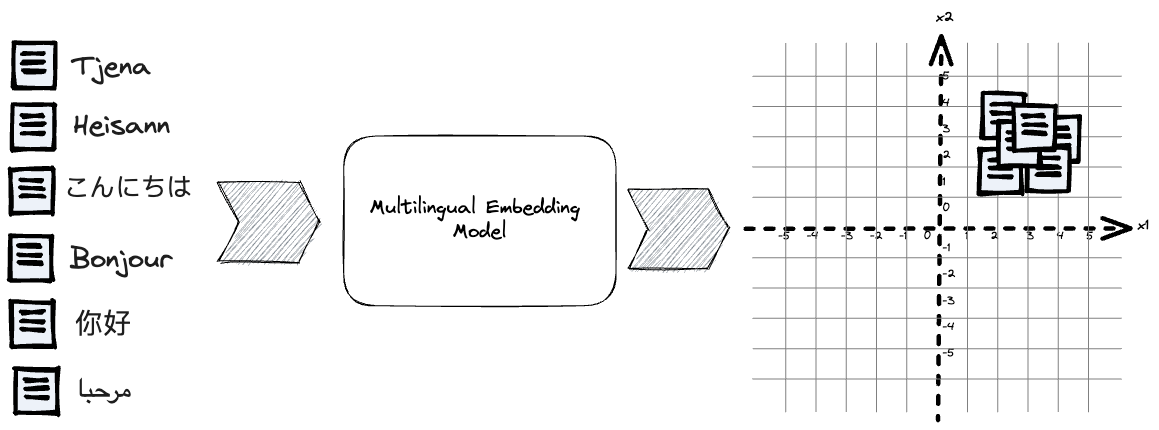
The fundamental concept behind text embedding models is transforming textual data into a continuous vector space, wherein similar items are brought closer together, and dissimilar ones are pushed farther apart. Mapping multilingual texts into a unified vector embedding space makes it possible to represent and compare queries and documents from various languages within this shared space. By using contrastive representation learning with retrieval data examples, we can make embedding representations useful for retrieval with nearest neighbor search.
A search system using embedding retrieval consists of two primary processes:
- Embedding inference, using an embedding model to map text to a point in a vector space of D dimensions.
- Retrieval in the D dimensional vector space using nearest neighbor search.
This blog post covers both aspects of an embedding retrieval system and how to accelerate them, while also paying attention to the task accuracy because what’s the point of having blazing fast but highly inaccurate results?
Transformer Model Inferencing
The most popular text embedding models are typically based on encoder-only Transformer models (such as BERT). We need a high-level understanding of the complexity of encoder-only transformer language models (without going deep into neural network architectures).
Inference complexity from the transformer architecture attention mechanism scales quadratically with input sequence length.
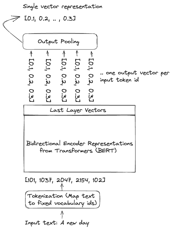
The BERT model has a typical input length limitation of 512 tokens, so the tokenization process truncates the input to avoid exceeding the architecture’s maximum length. Embedding models might also truncate the text at a lower limit than the theoretical limit of the neural network to improve quality and reduce training costs, as computational complexity is quadratic with input sequence length for both training and inference. The last pooling operation compresses the token vectors into a single vector representation. A common pooling technique is averaging the token vectors.
It’s worth noting that some models may not perform pooling and instead represent the text with multiple vectors, but that aspect is beyond the scope of this blog post.
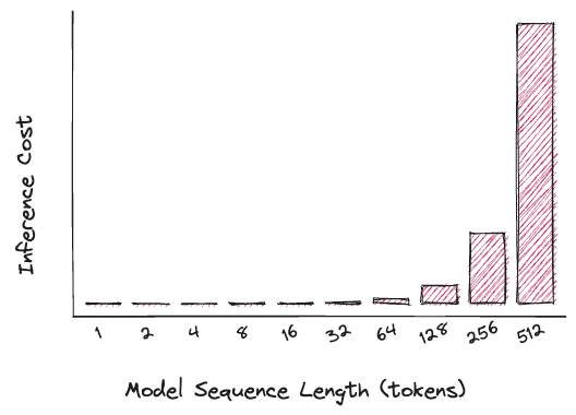
We use ‘Inference cost’ to refer to the computational resources required for a single inference pass with a given input sequence length. The graph depicts the relationship between the sequence length and the squared compute complexity, demonstrating its quadratic nature. Latency and throughput can be adjusted using different techniques for parallelizing computations. See model serving at scale for a discussion on these techniques in Vespa.
Why does all of this matter? For retrieval systems, text queries are usually much shorter than text documents, so invoking embedding models for documents costs more than encoding shorter questions.
Sequence lengths and quadratic scaling are some of the reasons why using frozen document-size embeddings are practical at scale, as it avoids re-embedding documents when the model weights are updated due to re-training the model. Similarly, query embeddings can be cached for previously seen queries as long as the model weights are unchanged. The asymmetric length properties can also help us design a retrieval system architecture for scale.
- Asymmetric model size: Use different-sized models for encoding queries and documents (with the same output embedding dimensionality). See this paper for an example.
- Asymmetric batch size: Use batch on-demand computing for embedding documents, using auto-scaling features, for example, with Vespa Cloud.
- Asymmetric compute architecture: Use GPU acceleration for document inference but CPU for query inference.
The final point is that reporting embedding inference latency or throughput without mentioning input sequence length provides little insight.
Choose your Fighter
When deciding on an embedding model, developers must strike a balance between quality and serving costs.
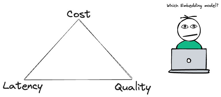
These serving-related costs are all roughly linear with model parameters and embedding dimensionality (for a given sequence length). For example, using an embedding model with 768 dimensions instead of 384 increases embedding storage by 2x and nearest neighbor search compute by 2x.
Accuracy, however, is not nearly linear, as demonstrated on the MTEB leaderboard.
| Model | Dimensionality | Model params (M) | Accuracy Average (56 datasets) | Accuracy Retrieval (15 datasets) |
| Small | 384 | 118 | 57.87 | 46.64 |
| Base | 768 | 278 | 59.45 | 48.88 |
| Large | 1024 | 560 | 61.5 | 51.43 |
In the following sections, we use the small E5 multilingual variant, which gives us reasonable accuracy for a much lower cost than the larger sister E5 variants. The small model inference complexity also makes it servable on CPU architecture, allowing iterations and development locally without managing GPU-related infrastructure complexity.
Exporting E5 to ONNX format for accelerated model inference
To export the embedding model from the Huggingface model hub to ONNX format for inference in Vespa, we can use the Transformer Optimum library:
$ optimum-cli export onnx --library transformers --task sentence-similarity -m intfloat/multilingual-e5-small model-dir
The above exports the model without any optimizations. The optimum client also allows specifying optimization levels, here using the highest optimization level usable for serving on the CPU.
The above commands export the model to ONNX format that can be imported and used with the Vespa Huggingface embedder. Using the Optimum generated ONNX and tokenizer configuration files, we configure Vespa with the following in the Vespa application package services.xml file:
<component id="e5" type="hugging-face-embedder">
  <transformer-model path="model/model.onnx"/>
  <tokenizer-model path="model/tokenizer.json"/>
</component>
These two simple steps are all we need to start using the multilingual E5 model to embed queries and documents with Vespa. We can also quantize the optimized ONNX model, for example, using the optimum library.
Quantization (post-training) converts the float32 model weights (4 bytes per weight) to byte (int8), enabling faster inference on the CPU.
Performance Experiments
To demonstrate the many tradeoffs, we assess the mentioned small E5 multilanguage model on the Swahili(SW) split from the MIRACL (Multilingual Information Retrieval Across a Continuum of Languages) dataset.
| Dataset | Language | Documents | Avg document tokens | Queries | Avg query tokens | Relevance Judgments |
| MIRACL sw | Swahili | 131,924 | 63 | 482 | 13 | 5092 |
We experiment with post-training quantization of the model (not the
output vectors) to document the impact quantization has on retrieval
effectiveness (NDCG@10).
We then study the serving efficiency gains (latency/throughput) on the same laptop-sized hardware using a quantized model versus a full precision model.
All experiments are run on an M1 Pro (arm64) laptop with 8 v-CPUs and 32GB of memory, using the open-source Vespa container image. No GPU acceleration and no need to manage CUDA driver compatibility, huge container images due to CUDA dependencies, or forwarding host GPU devices to the container.
- We use the multilingual-search Vespa sample application as the starting point for these experiments. This sample app was introduced in Simplify search with multilingual embedding models.
- We use the NDCG@10 metric to evaluate ranking effectiveness. When performing model optimizations, it’s important to pay attention to the impact on the task. This is stating the obvious, but still, many talk about accelerations and optimizations without mentioning task accuracy degradations.
- We measure the throughput of indexing text documents in Vespa. This includes embedding inference in Vespa using the Vespa Huggingface embedder, storing the embedding vector in Vespa, and regular inverted indexing of the title and text field. We use the vespa-cli feed option as the feeding client.
- We use the Vespa fbench tool to drive HTTP query load using HTTP POST against the Vespa query api.
- Batch size in Vespa embedders is one for document and query inference.
- There is no caching of query embedding inference, so repeating the same query text while benchmarking will trigger a new embedding inference.
Sample Vespa JSON formatted feed document (prettified) from the MIRACL dataset.
{
    "put": "id:miracl-sw:doc::2-0",
    "fields": {
        "title": "Akiolojia",
        "text": "Akiolojia (kutoka Kiyunani \u03b1\u03c1\u03c7\u03b1\u03af\u03bf\u03c2 = \"zamani\" na \u03bb\u03cc\u03b3\u03bf\u03c2 = \"neno, usemi\") ni somo linalohusu mabaki ya tamaduni za watu wa nyakati zilizopita. Wanaakiolojia wanatafuta vitu vilivyobaki, kwa mfano kwa kuchimba ardhi na kutafuta mabaki ya majengo, makaburi, silaha, vifaa, vyombo na mifupa ya watu.",
        "doc_id": "2#0",
        "language": "sw"
    }
}
| Model | Model size (MB) | NDCG@10 | Docs/second | Queries/second (*) |
| float32 | 448 | 0.675 | 137 | 340 |
| Int8 (Quantized) | 112 | 0.661 | 269 | 640 |
There is a small drop in retrieval accuracy from an NDCG@10 score
of 0.675 to 0.661 (2%), but a huge gain in embedding inference
efficiency. Indexing throughput increases by 2x, and query throughput
increases close to 2x. The throughput measurements are end-to-end,
either using vespa-cli feed or vespa-fbench. The difference in query
versus document sequence length largely explains the query and
document throughput difference (the quadratic scaling properties).
Query embed latency and throughput
Throughput is one way to look at it, but what about query serving latency? We analyze query latency of the quantized model by gradually increasing the load until the CPU is close to 100% utilization using vespa-fbench input format for POST requests.
/search/
{"yql": "select doc_id from doc where rank(doc_id contains \"71#13\",{targetHits:1}nearestNeighbor(embedding,q))", "input.query(q)": "embed(query:Bandari kubwa nchini Kenya iko wapi?)", "ranking": "semantic", "hits": 0}
The above query template tests Vespa end-to-end but does NOT perform a global nearest neighbor search as the query uses the rank operator to retrieve by doc_id, and the second operand computes the nearestNeighbor. This means that the nearest neighbor “search” is limited to a single document in the index. This experimental setup allows us to test everything end to end except the cost of exhaustive search through all documents.
This part of the experiment focuses on the embedding model inference and not nearest neighbor search performance. We use all the queries in the dev set (482 unique queries). Using vespa-fbench, we simulate load by increasing the number of concurrent clients executing queries with sleep time 0 (-c 0) while observing the end-to-end latency and throughput.
$ vespa-fbench -P -q queries.txt -s 20 -n $clients -c 0 localhost 8080
| Clients | Average latency | 95p latency | Queries/s |
| 1 | 8 | 10 | 125 |
| 2 | 9 | 11 | 222 |
| 4 | 10 | 13 | 400 |
| 8 | 12 | 19 | 640 |
As concurrency increases, the latency increases slightly, but not
much, until saturation, where latency will climb rapidly with a
hockey-stick shape due to queuing for exhausted resources.
In this case, latency is the complete end-to-end HTTP latency, including HTTP overhead, embedding inference, and dispatching the embedding vector to the Vespa content node process. Again, it does not include nearest neighbor search, as the query limits the retrieval to a single document.
Putting it all together - adding nearest neighbor search
In the previous section, we focused on the embedding inference throughput and latency. In this section, we change the Vespa query specification to perform an exact nearest neighbor search over all documents. This setup measures the end-to-end deployment, including HTTP overhead, embedding inference, and embedding retrieval using Vespa exact nearest neighbor search. With exact search, no retrieval error is introduced by using approximate search algorithms.
/search/
{"yql": "select doc_id from doc where {targetHits:10}nearestNeighbor(embedding,q)", "input.query(q)": "embed(query:Bandari kubwa nchini Kenya iko wapi?)", "ranking": "semantic", "hits": 10}
| Clients | Average latency | 95p latency | Queries/s |
| 1 | 18 | 20.35 | 55.54 |
| 2 | 19.78 | 21.90 | 101.09 |
| 4 | 23.26 | 26.10 | 171.95 |
| 8 | 32.02 | 44.10 | 249.79 |
With this setup, the system can support up to 250 queries/second
on a laptop with a 95 percentile below 50ms. If we don’t need to
support 250 queries/s but we want to lower serving latency, we can
configure Vespa to use multiple
threads
to evaluate the exact nearest neighbor search. More threads per
search allow parallelization of the exact nearest neighbor search
over several threads per query request. In this case, we allow Vespa
to distribute the search using four threads per query by adding
this tuning element to the
services.xml
configuration file:
<engine>
  <proton>
    <tuning>
      <searchnode>
        <requestthreads>
          <persearch>4</persearch>
        </requestthreads>
      </searchnode>
    </tuning>
  </proton>
 </engine>
The number of distance calculations (compute) per query stays the same, but by partitioning and parallelization of the workload, we reduce the serving latency.
| Clients | Average latency | 95p latency | Queries/s |
| 1 | 11.57 | 13.60 | 86.39 |
| 2 | 14.94 | 17.80 | 133.84 |
| 4 | 20.40 | 27.30 | 196.07 |
With this change, end-to-end serving latency drops from average
18ms to 11.6ms. Note that the thread per search Vespa setting does
not impact the embedding inference. Reducing serving latency is more important than maximizing the
throughput for many low-traffic use cases. The threads per search
setting allow making that tradeoff. It can also be handy if your
organization reserved instances from a cloud provider and your CFO
asks why the instances are underutilized while users complain about
high serving latency.
Putting it all together 2 - enabling approximate nearest neighbor search
Moving much beyond a corpus of 100k of documents, exact nearest neighbor search throughput is often limited by memory bandwidth - moving document corpus vector data to the CPU for similarity computations. By building approximate nearest neighbor search data structures during indexing, we can limit the number of vectors that need to be compared with the query vector, which reduces memory reads per query, lowers latency, and increases throughput by several orders of magnitude. So what’s the downside? In short:
- Adding approximate nearest neighbor (ANN) index structures increases resource usage during indexing and consumes memory in addition to the vector data.
- It impacts retrieval quality since the nearest neighbor search is approximate. A query might not retrieve the relevant documents due to the error introduced by the approximate search.
Retrieval quality degradation is typically measured and quantified using overlap@k, comparing the true nearest neighbors from an exact search with the nearest neighbors returned by the approximate search.
In our opinion, this is often overlooked when talking about embedding models, accuracy, and vector search. Speeding up the search with ANN techniques does impact retrieval quality. For example, entries on the MTEB leaderboard are certainly not using any approximation, so in practice, the results will not be as accurate if deployed using approximate vector search techniques.
In the following, we experiment with Vespa’s three HNSW indexing parameters and observe how they impact NDCG@10. This setup is a slightly unusual experimental setup since instead of calculating the overlap@10 between exact and approximate, we are using the NDCG@10 retrieval metric directly. In the context of dense text embedding models for search, we believe this experimental setup is the best as it allows us to quantify the exact impact of introducing approximate search techniques.
There are two HNSW index time parameters in Vespa. Changing any of those requires rebuilding the HNSW graph, so we only test with two permutations of these two parameters. For each of them, we run an evaluation with a query time setting, which explores more nodes in the graph, making the search more accurate (at the cost of more distance calculations).
The query time hnsw.exploreAdditionalHits is an optional parameter of the Vespa nearestNeighbor query operator, and the hnsw index time settings are configured in the schema.
{"yql": "select doc_id from doc where {targetHits:10, hnsw.exploreAdditionalHits:300}nearestNeighbor(embedding,q)", "input.query(q)": "embed(query:Je, bara Asia lina visiwa vingapi?)", "ranking": "semantic", "hits": 10}
| max-links-per-node | neighbors-to-explore-at-insert | hnsw.exploreAdditionalHits | NDCG@10 |
| 16 | 100 | 0 | 0.5115 |
| 16 | 100 | 100 | 0.6415 |
| 16 | 100 | 300 | 0.6588 |
| 32 | 500 | 0 | 0.6038 |
| 32 | 500 | 100 | 0.6555 |
| 32 | 500 | 300 | 0.6609 |
As the table above demonstrates, we can reach the same NDCG@10 as
the exact search by using max-links-per-node 32,
neighbors-to-explore-at-insert 500, and hnsw.exploreAdditionalHits 300.
The high hnsw.exploreAdditionalHits setting indicates that we could
alter the index time settings upward, but we did not experiment
further. Note the initial HNSW setting in row 1 and the significant
negative impact on retrieval quality.
As a rule of thumb, if increasing hnsw.exploreAdditionalHits hits
a plateau in either overlap@k or the end metric we are optimizing
for; it’s time to look at increasing the quality of the HNSW graph
by increasing the index time settings (max-links-per-node and
neighbors-to-exlore-at-insert).
With retrieval accuracy retained, we can use those HNSW settings to re-evaluate the serving performance of both indexing and queries and compare it with exact search (where we did not have to evaluate the accuracy impact).
Without HNSW structures, we could index at 269 documents/s. With HNSW (32,500), indexing throughput drops to 230 documents/s. Still, most of the cost is in the embedding inference part, but there is a noticeable difference. The relative change would be larger if we just evaluated indexing without embedding inference.
| Clients | Average latency | 95p latency | Queries/s |
| 1 | 12.78 | 15.80 | 78.20 |
| 2 | 13.08 | 15.70 | 152.83 |
| 4 | 15.10 | 18.10 | 264.89 |
| 8 | 19.66 | 28.90 | 406.76 |
After introducing HNSW indexing for approximate search, our laptop-sized deployment can support 400 QPS (compared to 250 with exact search) with a 95 percentile latency below 30 ms.
Summary
Using the open-source Vespa container image, we’ve delved into exploring and experimenting with both embedding inference and retrieval right on our laptops. The local experimentation, avoiding specialized hardware acceleration, holds immense value, as it eliminates prolonged feedback loops.
Moreover, the same Vespa configuration files suffice for many deployment scenarios, be it in on-premise setups, on Vespa Cloud, or locally on a laptop. The beauty lies in the fact that specific infrastructure for managing embedding inference and nearest neighbor search as separate infra systems becomes obsolete with Vespa’s native embedding support.
Within this blog post, we’ve shown how applying post-training quantization to embedding models yields a substantial improvement in serving performance without significantly compromising retrieval quality. Subsequently, our focus shifted towards embedding retrieval with nearest neighbor search. This allowed us to explore the tradeoffs between exact and approximate nearest neighbor search methodologies.
A noteworthy advantage of executing embedding inference within Vespa locally lies in the proximity of vector creation to the vector storage. To put this into perspective, consider the latency numbers in this post versus procuring an embedding vector in JSON format from an embedding API provider situated on a separate continent. Transmitting vector data across continents commonly incurs delays of hundreds of milliseconds.
If you are interested to learn more about Vespa; See Vespa Cloud - getting started, or self-serve Vespa - getting started. Got questions? Join the Vespa community in Vespa Slack.