UPDATE 2023-06-06: use new syntax to configure Bert embedder.

Photo by fabio on Unsplash

Deep-learned embeddings are popular for search and recommendation use cases, and organizations must manage and operate these embeddings efficiently in production. One emerging strategy which reduces embedding lifecycle complexity is to use frozen models which output frozen foundational embeddings that are reusable and customizable for different tasks.

This post introduces the concept of using reusable frozen embeddings and tailoring them with Vespa.

Background

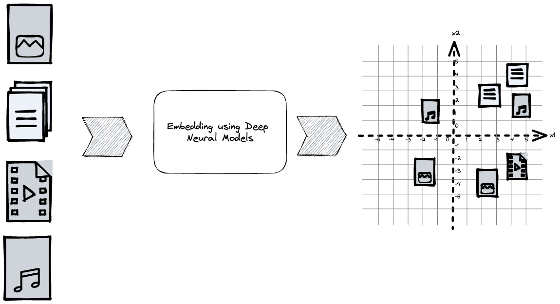
Encoding data objects using deep learning models allows for representing objects in a high-dimensional vector space. In this latent embedding vector space, one can compare the objects using vector distance functions, which can be used for search, recommendation, classification, and clustering. There are three primary ways developers can introduce embedding representations of data in their applications:

• Using commercial embedding providers
• Using off-the-shelf open-source embedding models
• Training custom embedding models

All three incur training and inference (computational) costs, which are proportional to the model size, the number of objects, and the object input sizes. In addition, the output vector embedding must be stored and potentially indexed for efficient retrieval.

Operating and maintaining embeddings in production #MLEmbeddingOps

Suppose we want to modify an embedding model by fine-tuning it for a task or replacing it with a new model with a different vector dimensionality. Then, all our data objects must be reprocessed and embedded again. Reprocessing for any model change might be easy for small-scale applications with a few million data points. Still, it quickly gets out of hand with larger-scale evolving datasets in production.

Consider a case where we have an evolving dataset of 10M news articles that we have implemented semantic search for, using a model that embeds query and document texts into vector representations. Our search service has been serving production traffic for some time, but now the ML team wants to change the embedding model. Now, to get this new model into production for online evaluation, we roughly need to follow these steps:

• Run inference with the new model over all documents in the index to obtain the new vector embedding. This stage requires infrastructure to run inferences with the model or pay an embedding inference provider per inference. We must also serve the current embedding model, which is in production, used to embed new documents and the current real-time stream of queries.

• Index the new vector embedding representation to our serving infrastructure used for efficient vector search. Suppose, we are fortunate enough to be using Vespa, which supports multiple embedding fields per document schema. In that case, we can index the new embedding in a new field without duplicating other fields and creating an entirely new schema or index. Adding the new tensor field still adds to the serving cost, as we double the resource usage footprint related to indexing and storage.

• After all this, we are finally ready to evaluate the new embedding model online. Depending on the outcome of the online evaluation, we can garbage collect either the new or old embedding field.

That’s a lot of complexity and cost to evaluate a model online, but now we can relax. But, wait, our PM now wants to introduce news article recommendations for the home page, and the ML team is planning on using embeddings for this project. We also hear they are discussing a related articles feature they want to launch soon.

Very quickly we will face the challenge of maintaining and operating three different embedding-based use cases, each with model iterations, and going through the above process. There must be a better way. What if we could somehow reuse the embeddings for multiple tasks?

Frozen embeddings to the rescue

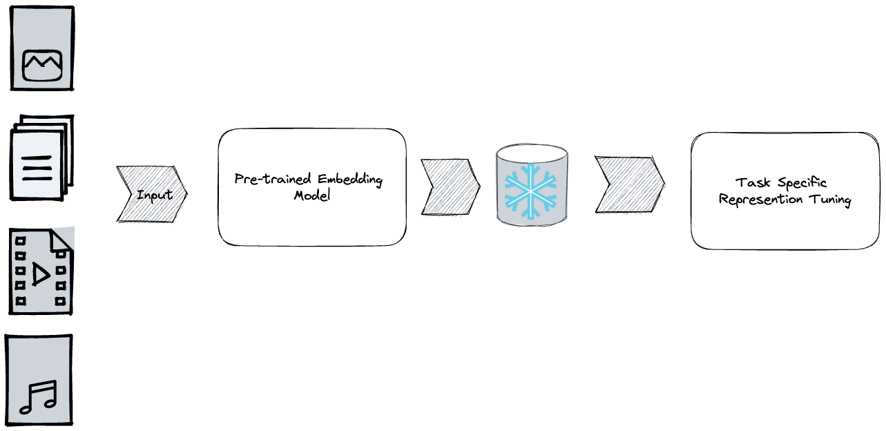
An emerging industry trend that helps reduce #MLEmbeddingOps complexity is to use frozen foundational embeddings that can be reused for different tasks without incurring the usual costs related to embedding versioning, storage, inference, and training.

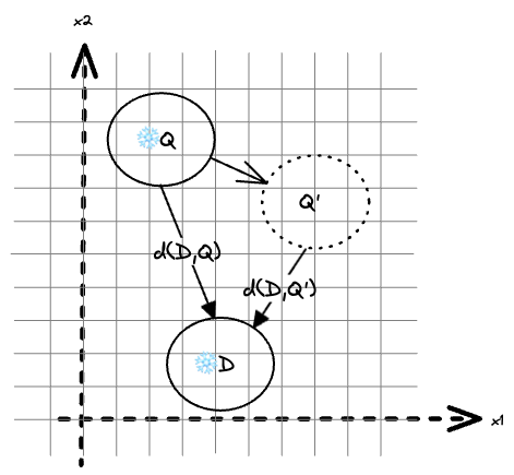
A frozen model embeds data Q and D into vector space. By transforming the Q representation to Q’, the vector distance is reduced (d(D,Q') < d(D,Q). This illustrates fine-tuning of metric distances over embeddings from frozen models. Note that the D representation does not change, which is a practical property for search and recommendation use cases with potentially billions of embedding representations of items.

With frozen embeddings from frozen models, the data is embedded once using a foundational embedding model. Developers can then tailor the representation to specific tasks by adding transformation layers. The fixed model will always produce the same frozen embedding representation for the same input. So as long as the input data does not change, we will not need to invoke the model again. In our news search example, we can use the same frozen document embeddings for all three use cases.

The following sections describe different methods for tailoring frozen embeddings for search or recommendation use cases.

• Tuning the query tower in two-tower embedding models
• Simple query embedding transformations
• Advanced transformations using Deep Neural Networks

Two-tower models

The industry standard for semantic vector search is using a two-tower architecture based on a Transformer based model.

This architecture is also called a bi-encoder model, as there is a query and document encoder. Most of the two-tower architecture models use the same weights for both the query and document encoder. This is not ideal as if we tune the model, we would need to reprocess all our items again. By de-coupling the model weights of the query and document tower, developers can treat the document tower as frozen. Then, when fine-tuning the model for the specific task, developers tune the query tower and freeze the document tower.

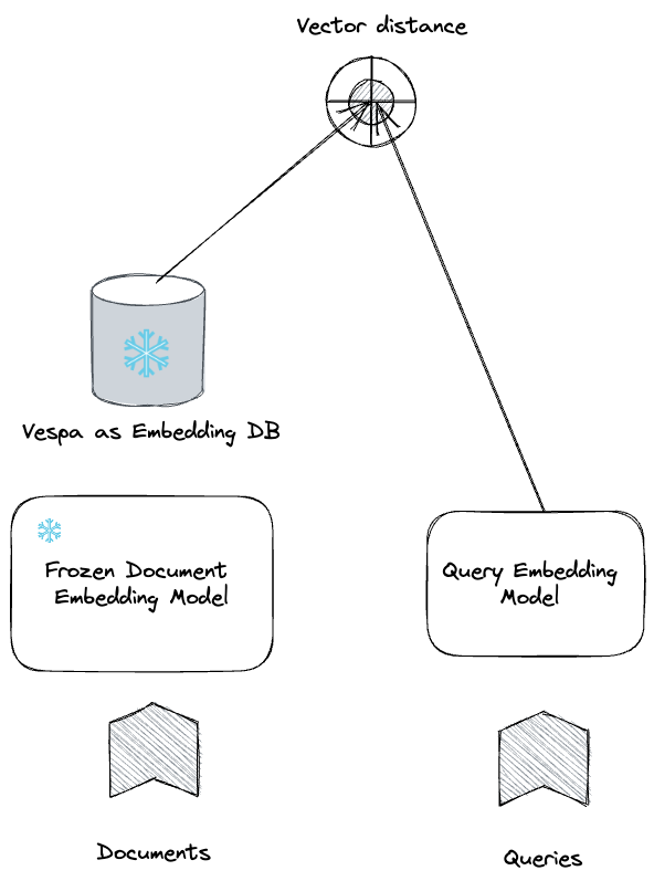
The frozen document tower and corresponding embeddings significantly reduce the complexity and cost of serving and training. For example, during training, there is no need to encode the document in the training data, it can be fetched directly from Vespa. This saves at least 2x of computational complexity during training. In practice, since documents are generally longer than queries and Transformer models scale quadratic with input lengths, the computational saving is higher than that.

On the serving side in Vespa, there is no need to re-process the documents, as the same input will produce the exact same frozen document embedding representation. This saves the compute of performing the inference and avoids introducing new embedding fields or embedding versioning. And, because Vespa allows deploying multiple query tower models, applications may test the accuracy of new models, without re-processing documents, which allows for frequent model deployment and evaluations.

Managing complex infrastructure for producing text embedding vectors could be challenging, especially at query serving time, with low latency, high availability, and high query throughput. Vespa allows developers to represent embedding models in Vespa. Consider the following schema, expressed using Vespa’s schema definition language:

schema doc {
  document doc {
    field text type string {}  
  } 
  field embedding type tensor<float>(x[384]) { 
    indexing: input text | embed frozen | attribute | index
  }
}

In this case, Vespa will produce embeddings using a frozen embedding model, and at query time, we can either use the frozen model to encode the query or a new fine-tuned model. Deploying multiple query tower models allows for query time A/B testing which increases model deployment velocity and shortens the ML feedback loop.

curl \
 --json "
  {
   'yql': 'select text from doc where {targetHits:10}nearestNeighbor(embedding, q)',
   'input.query(q)': 'embed(tuned, dancing with wolves)' 
  }" \
 https://vespaendpoint/search/

The first argument of the embed command is the model to use when encoding the query.
For each new query tower model, developers will add the model to a directory in the Vespa application package, and give it a name, which is referenced at query inference time.

Re-deployment of new models is a live change, where Vespa automates the model distribution to all the nodes in the cluster, without service interruption or downtime.

<component id="frozen" type="bert-embedder">
    <transformer-model path="models/frozen.onnx"/>
    <tokenizer-vocab path="models/vocab.txt"/>
</component>

<component id="tuned" type="bert-embedder">
    <transformer-model path="models/tuned.onnx"/>
    <tokenizer-vocab path="models/vocab.txt"/>
</component>

Snippet from the Vespa application services.xml file, which defines the models and names, see represent embedding models for details. Finally, how documents are ranked is expressed using Vespa ranking expressions.

rank-profile default inherits default {
  inputs {
    query(q) tensor<float>(x[384])
  }
  first-phase {
    expression: cos(distance(field,embedding))
  }
}

Simple embedding transformation

Simple linear embedding transformation is great for the cases where developers use an embedding provider and don’t have access to the underlying model weights. In this case tuning the model weights is impossible, so the developers cannot adjust the embedding model towers. However, the simple approach for adapting the model is to add a linear layer on top of the embeddings obtained from the provider.

The simplest form is to adjust the query vector representation by multiplying it with a learned weights matrix. Similarly to the query tower approach, the document side representation is frozen. This example implements the transformation using tensor compute expressions configured with the Vespa ranking framework.

rank-profile simple-similarity inherits default {
  constants {
    W tensor<float>(w[128],x[384]): file: constants/weights.json
  }
 
  function transform_query() {
     expression: sum(query(q) * constant(W), w)   
  }

  first-phase {
    expression: attribute(embedding) * transform_query()
  }
}

The learned weights are exported from any ML framework (e.g., PyTorch, scikit-learn) used to train the matrix weights. And the weights are exported to a constant tensor file. Meanwhile, the transform_query function performs a vector -matrix product, returning a modified vector of the same dimensionality.

This representation is then used to score the documents in the first-phase ranking expression. Note that this is effectively represented as a re-ranking phase as the query tensor used for the nearestNeighbor search is untouched.

The weight tensor does not necessarily need to be a constant across all users. For example, one can have a weight tensor per user, as shown in the recommendation use case, to unlock true personalization.

Advanced transformation using Deep Neural Networks

Another approach for customization is to use the query and document embeddings as input to another Deep Neural Network (DNN) model. This approach can be combined with the previously mentioned approaches because it’s applied as a re-scoring model in a phased rankingpipeline.

import torch.nn as nn
import torch
class CustomEmbeddingSimilarity(nn.Module):
	def __init__(self, dimensionality=384):
		super(CustomEmbeddingSimilarity, self).__init__()
		self.fc1 = nn.Linear(2*dimensionality, 256)
		self.fc2 = nn.Linear(256, 128)
		self.fc3 = nn.Linear(128, 64)
		self.fc4 = nn.Linear(64, 1)
	def forward(self, query , document):
		x = torch.cat((query, document), dim=1)
		x = nn.functional.relu(self.fc1(x))
		x = nn.functional.relu(self.fc2(x))
		x = nn.functional.relu(self.fc3(x))
		return torch.sigmoid(self.fc4(x))
dim = 384
ranker = CustomEmbeddingSimilarity(dimensionality=dim)
# Train the ranker model ..
# Export to ONNX for inference with Vespa 
input_names = ["query","document"]
output_names = ["similarity"]
document = torch.ones(1,dim,dtype=torch.float)
query = torch.ones(1,dim,dtype=torch.float)
args = (query,document)
torch.onnx.export(ranker,
                  args=args,
                  f="custom_similarity.onnx",
                  input_names = input_names,
                  output_names = output_names,
                  opset_version=15)

The above PyTorch model.py snippet defines a custom DNN-based similarity model which takes the query and document embedding as input. This model is exported to ONNX format for accelerated inference using Vespa’s support for ranking with ONNX models.

rank-profile custom-similarity inherits simple-similarity {
  function query() {
    # Match expected tensor input shape
    expression: query(q) * tensor<float>(batch[1]):[1]
  }
  function document() {
    # Match expected tensor input shape
    expression: attribute(embedding) * tensor<float>(batch[1]):[1]
  }
  onnx-model dnn {
    file: models/custom_similarity.onnx
    input "query": query
    input "document": document
    output "similarity": score
  }
  second-phase {
    expression: sum(onnx(dnn).score)
  }
}

This model might be complex, so one typically use it as a second-phase expression, only scoring the highest ranking documents from the first-phase expression.

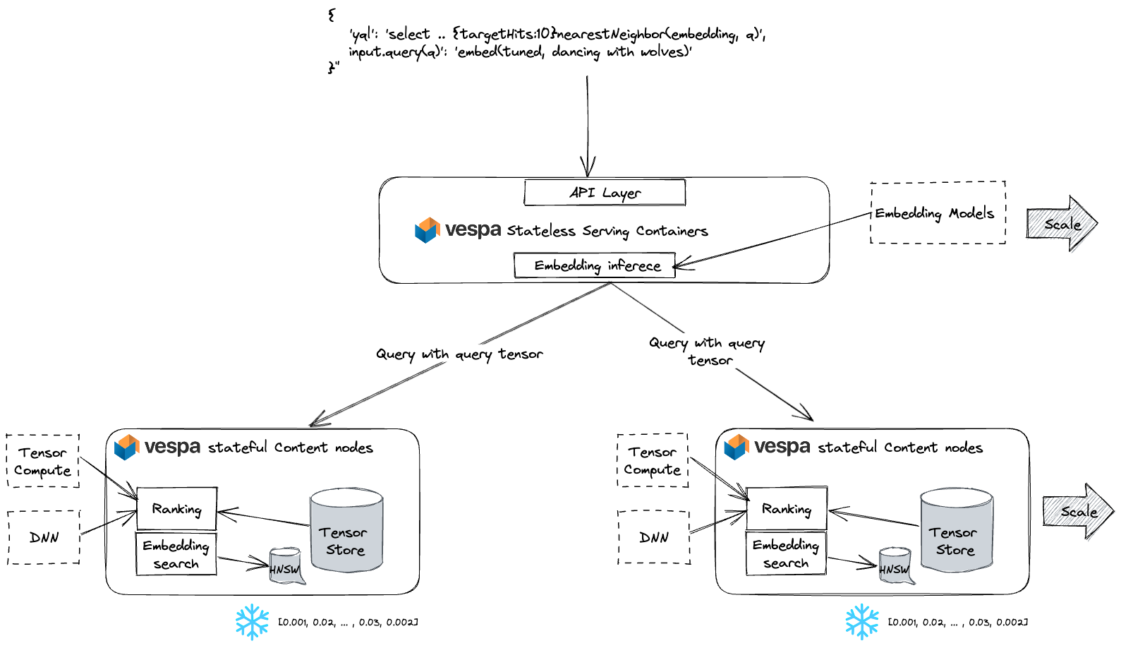
The Vespa serving architecture operates in the following manner: The stateless containers performs inference using the embedding model(s). The containers are stateless, which allows for fast auto-scaling with changes in query and inference volume. Meanwhile, the stateful content nodes store (and index) the frozen vector embeddings. Stateful content clusters are scaled elastically in proportion to the embedding volume. Additionally, Vespa handles the deployment of ranking and embedding models.

Summary

In this post, we covered three different ways to use frozen models and frozen embeddings with Vespa while still allowing for task-specific customization of the embeddings or the similarity function.

Simplify your ML-embedding use cases by getting started with the custom embeddings sample application. Deploy the sample application locally using the Vespa container image or to Vespa Cloud. Got questions? Join the community in Vespa Slack.