
If you have a Solr background, Vespa might look interesting for all its modern search capabilities. For example:
- Tensor support for vector search as well as recommendations.
- Integration with embedding models and LLMs.
- Flexible ranking.
At least that’s what sparked my interest (I came to Vespa from a Solr&Elasticsearch background). This, plus the performance and scalability dimensions.
Performance-wise, Vespa trades some of the initial write speed for much faster queries. Search performance gains tend to be higer when queries are more complex, like in the case of vector search and even more so when dealing with multiple vectors (e.g., ColBERT and ColPali). Have a look at the Vespa vs Elasticsearch performance comparison report for some reference numbers that will mostly hold for Solr as well.
Vespa is used at massive scale, for example:
- Web-scale search (e.g., Perplexity).
- Enterprise search (e.g., Yahoo).
- E-commerce search and recommendations (e.g., Vinted).
To scale horizontally, Vespa uses virtual buckets, which means you don’t have to worry about over-sharding or splitting shards as you scale out. Hot-spots are a very rare sight in Vespa. For more details, here’s a presentation about Vespa’s architecture compared to Solr’s (and Elasticsearch’s) with the corresponding slides.
If this sounds interesting, your next question might be: will Vespa work well for my use case?
As with everything, it’s about the details. But this post will give you a good starting point, since we’ll cover different facets of Solr’s functionality (pun intended 😅) and see how Vespa does it:
- Schema and configuration. Because we need to prepare the engine for data and queries.
- Writes. How writes and updates work.
- Lexical search. How Vespa deals with tokenization and ranking on tokens.
- Faceting. Solr has lots of approaches here; let’s see the Vespa equivalents.
- Vector search. This is where Vespa shines due to its tensor support, so we’ll cover multiple aspects:
- Intro to tensors via a recommendation example
- Semantic search with tensors
- Combining vector with lexical search
- Multiple vectors per document
- Plugin points. Many Solr deployments are extended with custom code. Let’s see how to do that in Vespa.
Let’s start with the setup and build from there.
Schema and configuration
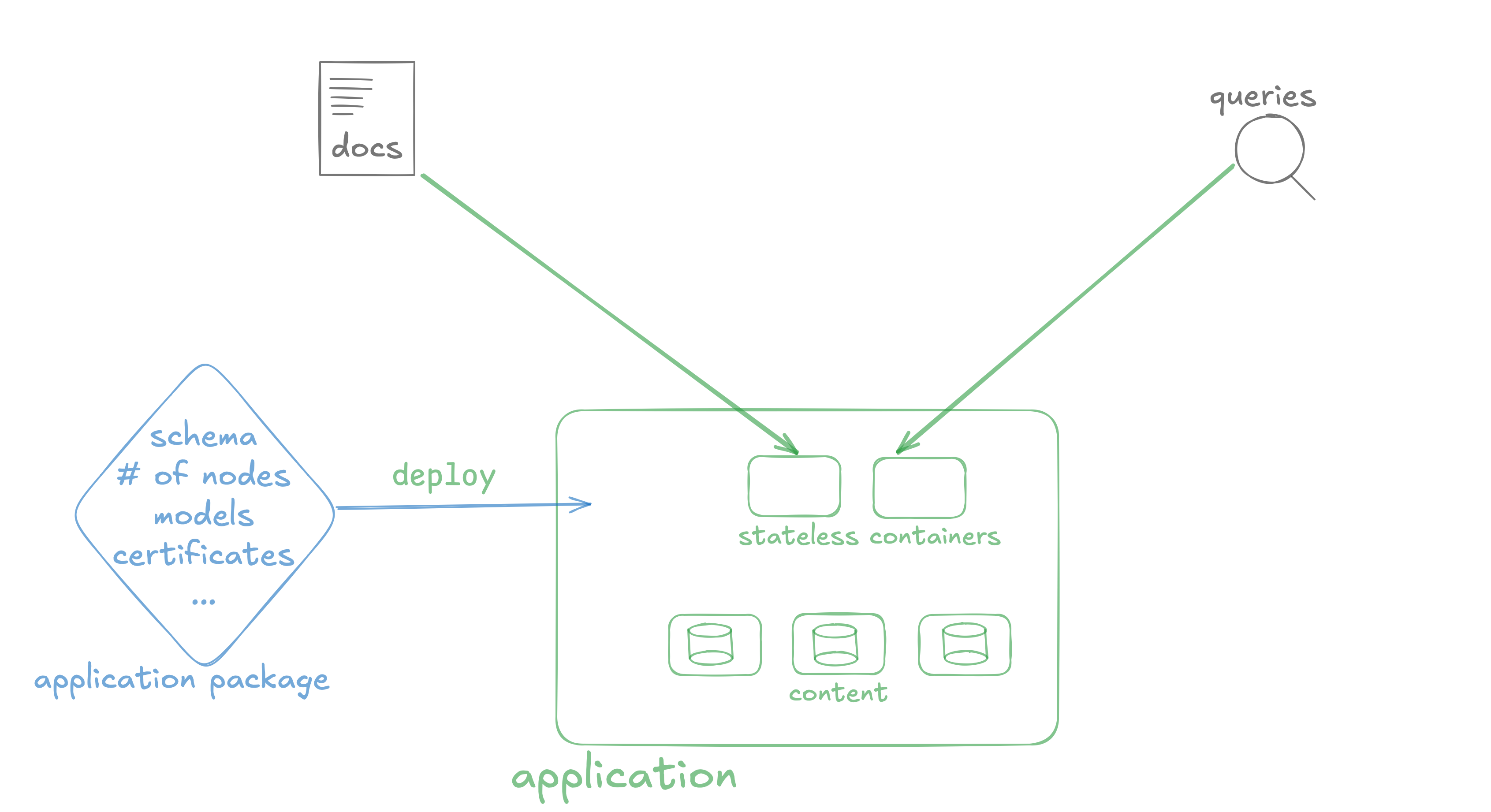
Before you write to Vespa, you need an application package. The application package contains all the configuration, from the schema to JVM memory settings and even the number of nodes. There’s some overlap with Solr’s configsets, but an application package would also include options that would normally go in solr.xml or solr.in.sh.
Note: You can find a “dictionary” between Vespa concepts (like application package) and their Solr/Elasticsearch/OpenSearch counterparts here.
When you start Vespa locally (e.g., using Docker/Podman), Vespa nodes that hold data (content nodes) and those that run queries (container nodes) are not started yet. They start only when you deploy the application package: because now they know their settings, which node should run on which host, etc.
It’s a similar process with Vespa Cloud: your nodes start (and you start paying for them) only when you deploy the application package.
You’d normally deploy the application package using the Vespa CLI:
# use --wait to show deployment logs in the terminal
# otherwise, Vespa CLI exists and deployment is done in the background
vespa deploy --wait 900
Schema
Besides the different format, most Solr schema elements have a direct equivalent in Vespa. Let’s take this example:
  <fields>
    <field name="id" type="string" indexed="false" stored="true"/>
    <field name="title" type="text_general" indexed="true" stored="true"/>
    <field name="price" type="int" indexed="true" docValues="true" stored="true"/>
  </fields>
The Vespa equivalent is:
schema my_document_type {
  document my_document_type {
    field id type string {
      indexing: attribute | summary
    }
    field title type string {
      indexing: index | summary
    }
    field price type int {
      indexing: attribute | summary
      attributes: fast-search
    }
  }
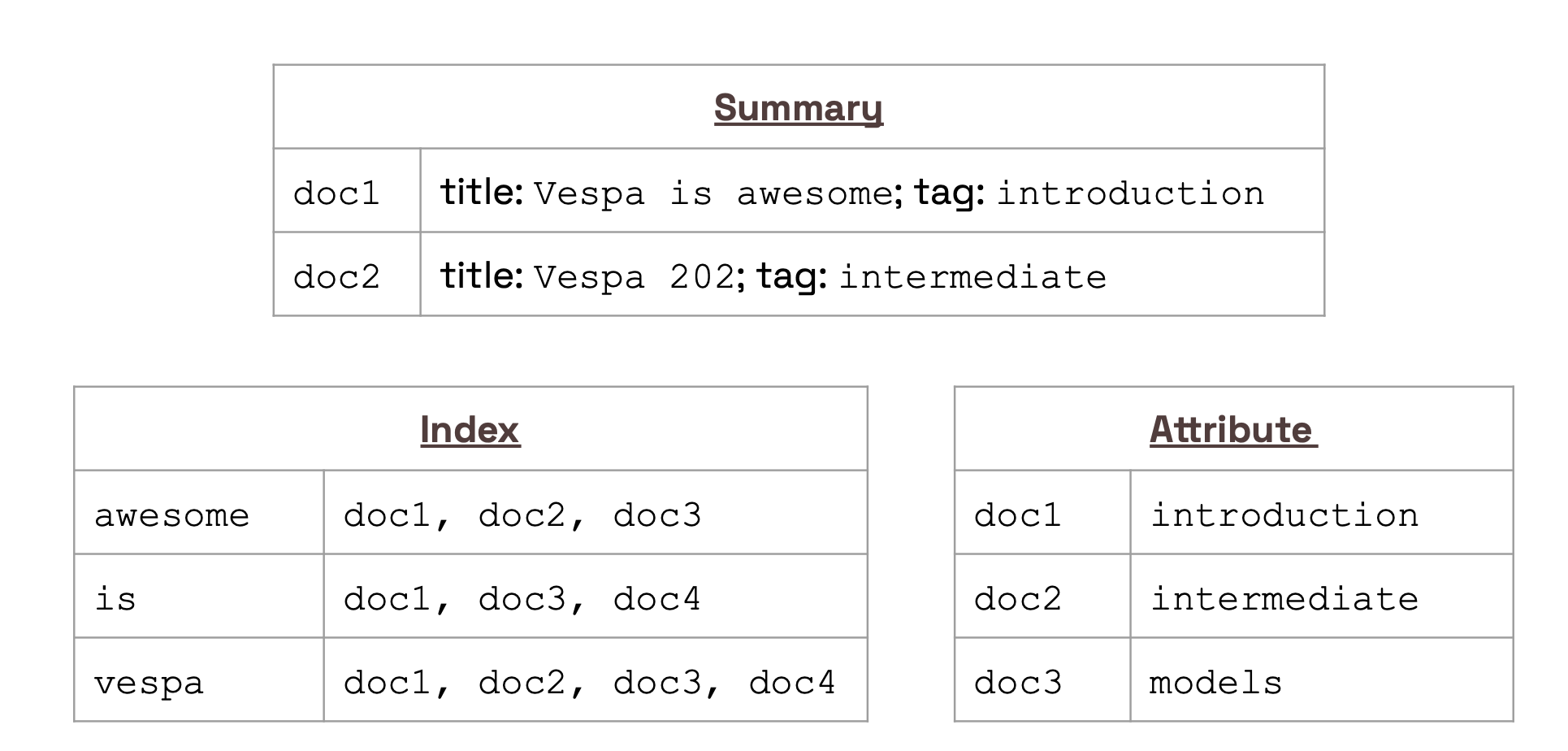
Core types, such as string and integer, are equivalent. Their options have different names, but the functionality behind them is similar:
- attribute means that a field is written as is (not tokenized). By default, attributes are loaded in memory (can also be paged to disk) so they can be used for ranking. Think of attributes as docValues in Solr.
- summary is similar to stored in Solr.
- index fields are tokenized and indexed, quite close to our
text_generalwithindex="true"in Solr. - fast-search is also indexing attributes (like
index="true"in Solr).
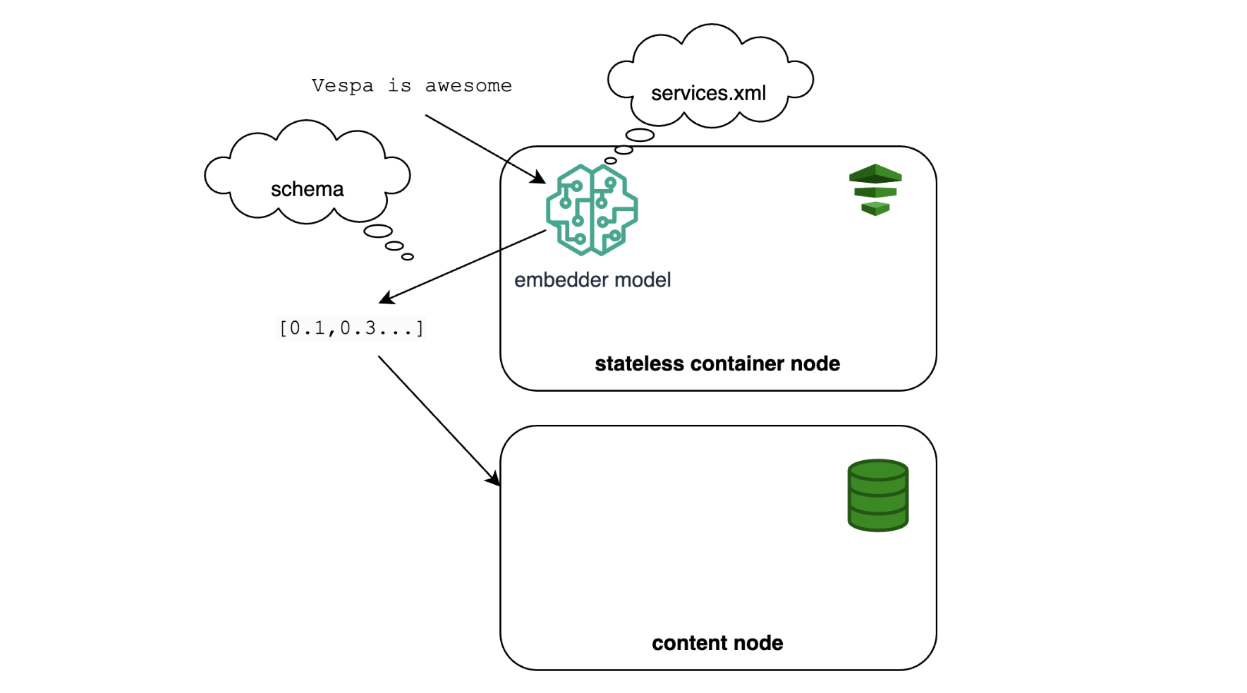
If we change summary to stored and attribute to docValues, this diagram may look very familiar:
Not everything is the same, though. Most importantly, tokenization won’t have the same defaults. Vespa will, for example, detect language and do the appropriate stemming out of the box. Check out the linguistics documentation for more details. If you tweaked your analysis with a lot of effort, I have good news: you can port most of your Solr analyzers to Vespa via Lucene linguistics.
Beyond the example schema above, you might be missing dynamic fields from Solr. Vespa’s schema is static, but you can implement similar functionality with maps. A map will allow arbitrary keys and will work for search and grouping/faceting. We’ll expand on grouping below.
You can’t use maps for ranking, for example if you want to take a numeric value and use it as a boost. For that, you can use tensors, which can also hold arbitrary keys. We’ll expand on tensors below as well. But before that, let’s look at how you can write to Vespa.
Writes
There might be some terminology clash here: “indexing” in Solr is called “feeding” in Vespa. Both terms refer to writing, which can be creating or updating documents.
Vespa’s document/v1 API is very similar to Solr’s /update handler. At least when it comes to writes. Here’s an example request:
curl -X POST -H "Content-Type:application/json" --data '
  {
      "fields": {
          "title": "Hello world",
          "price": 100
      }
  }' \
  http://localhost:8080/document/v1/my_namespace/my_document_type/docid/my_document_id
Where:
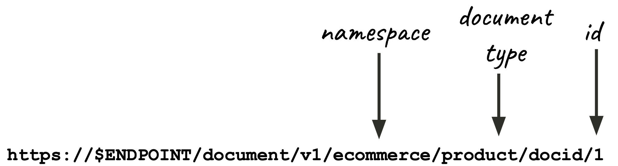
my_document_idis the unique ID that you also use in Solr. In Vespa, you don’t have to put it in the schema. But in this case, you can’t do full-text search on it, either.my_namespaceis a virtual separation of documents, typically used to avoid duplicate IDs. For example, if you have documents from two sources that produce their own IDs (which may clash), put them in different namespaces. You can still search them all together.my_document_typerefers to a physical separation of documents with a corresponding schema. Very similar to Solr’s collections.- The JSON representation of the document goes under the
fieldskey.
The order of metadata in the document V1 API is namespace, document type, document ID, like so:
With this translation in mind, you can look at other request types and probably find them similar. An in-place update, for example:
curl -X POST -H "Content-Type:application/json" --data '
  {
      "fields": {
        "price": {
          "assign": 101
        }
      }
  }' \
  http://localhost:8080/document/v1/my_namespace/my_document_type/docid/my_document_id
Or a delete-by-query. Here’s one removing all data (selection=true, more on document selection expressions here) in a cluster+namespace+document type combination:
curl -X DELETE \
  "http://localhost:8080/document/v1/my_namespace/my_document_type/docid?selection=true&cluster=my_cluster"
Note: The
clustervalue is defined inservices.xmlunder thecontentsection. Content nodes are like Solr’s data nodes - they hold data. By contrast, container nodes are like Solr’s coordinator nodes - they process query and write requests. In Vespa, they are always separate processes, because container nodes run in the JVM, while content nodes run compiled binaries (most importantly, proton).
Back to the writes themselves, there are good news and bad news. The bad news is that you can’t batch. You can achieve high write throughput via HTTP/2. The Vespa CLI and FeedClient work on HTTP/2 out of the box. Think of FeedClient as SolrJ - at least as far as writes are concerned.
The flipside is… well, there are two 🙂 One is that you don’t have to deal with partially failed batches: even if HTTP/2 operations are async, it’s pretty straightforward to handle failures. Here’s how Logstash’s Vespa output does it. Speaking of Logstash, it’s a good tool to write data to Vespa, here’s a tutorial for 5 use-cases. If you’re just getting started, Logstash can also generate an application package (including the schema) based on your data. Full tutorial here.
Secondly, Vespa’s writes are real-time: once you get an API response from the request, the document is available for search. No need for soft-commits, though Vespa has a hard commit equivalent: flush. A side-benfit of real-time writes is that updates are much faster: no need to look up the transaction log to get the latest document version. Attribute fields can be updated in place (like in Solr), but that is also faster because Vespa doesn’t have to rewrite the whole segment’s docValues, it’s a proper in-place update.
Assuming we have some data in Vespa, let’s move on to searches.
Lexical search
Most of the query documentation examples will show Vespa Query Language (YQL), which seems like a cross between SQL and Solr’s Lucene Query Parser. For example:
- To select everything:
select * from sources * where true - Search a document type (i.e., a collection in Solr) for a word in a field:
select * from my_document_type where title contains "hello" - Boolean query:
select * from my_document_type where title contains "hello" AND price > 100
You’ll find equivalents for more exotic queries, too. For example, geo search or the terms query parser. As with Solr, there are different syntax options. Besides YQL, you can use the Select syntax, similar to Solr’s JSON Query DSL. Or the Simple Query Language, which has no equivalent in Solr, but it’s designed to be more user-facing, much like Elasticsearch’s Simple Query String.
Ranking
Like Solr, Vespa will - by default - return the top 10 hits sorted by relevance. You can change things like paging via query parameters, like in Solr. These query parameters can also go into the JSON body of the request, similar to Solr’s JSON Request API.
Vespa supports BM25, but the default scoring is done with nativeRank, which trades off some query performance for better relevance. For example, based on token position (the earlier a token appears in a document, the better) and proximity (the closer tokens are to each other, the better).
Like Solr, in Vespa you can customize the ranking function. In fact, customized ranking is where Vespa shines. Here are a few reasons:
- Ranking functions can be arbitrarily complex. You have a wide range of input data (rank features) and transformations (ranking expressions) to choose from.
- You can (and probably should) use tensors for ranking. We’ll expand on tensors below, but if you look at the Tensor Guide, you’ll see that you can encode things like user preferences in them, which you can use for boosting. This is both fast and powerful.
- You can use different ML models for ranking and re-ranking (e.g., Learning to Rank). You can use pretty much any ONNX model, cross-encoders and more.
- Expensive ranking can also be fast. You can configure the number of threads per search and distribute the ranking work across multiple nodes.
- Ranking happens in 3 configurable phases. The first phase will rank all matching documents. The second phase re-ranks the top N results per content node, typically with a more expensive algorithm. The third phase happens on the container node that runs the query, after it gathers results from content nodes. More details here.
In Vespa, most of the ranking logic is defined in the rank profile, which is part of the schema, not in query parameters. By contrast, in Solr, you can do both query parameters and request handler defaults. Vespa is more opinionated here, which might requires some getting used to, if you’re a query-parameters kind of person.
Note: Like with Solr, query latency won’t drop linearly with the number of content nodes, because there’s the scatter-gather overhead. In practice, that overhead seems smaller, because it’s common to use 10-20 content nodes for a search without noticing inefficiencies. Especially if queries are complex. With Solr, if you want to optimize for query throughput, you really want to keep that number down, preferably to 1.
In short, you’re covered for lexical search and ranking 🙂 But surely you’re using some sort of facets, so let’s move on to that.
Faceting
While Solr has a lot of approaches to faceting, Vespa only has grouping, with two syntax variants:
- The YQL variant, in the form of
select $EXPRESSION | $GROUPING_EXPRESSION. - The Select variant, which adds a
groupingkey to the JSON request body, underselect.
The first variant is more concise, but the second one can be easier to build programmatically.
Functionally, grouping is similar to Solr’s JSON Facet API, in that it supports nested facets indefinitely (within hardware limits).
Grouping in Vespa can also act like grouping in Solr, in the sense that you can use it for field collapsing. Like Solr, which has result grouping and the Collapsing Query Parser for this, Vespa has an alternative approach: diversity in the rank profile.
Note: at the time of writing this, Vespa’s grouping always runs on top of query results. If you need to change the facet domain, you’ll need to run a separate query. This is typically cheap&cached and can be automated via a custom searcher.
Solr also has streaming expressions, which Vespa doesn’t have yet. But the main blocks are there:
- You can stream data from content nodes through visiting
- You can build custom components in the container nodes to write your own logic on top of that data. Or you can process it outside Vespa.
We’ll discuss custom components towards the end. For now, let’s move on to vector search.
Vector search
Chances are, tensor support is the main reason you’re here. Vespa had tensor support since 2014 (yes, it’s not a typo, it’s been 10+ years). There’s a lot of cool functionality to cover here, but we’ll focus on three main areas:
- Intro to tensors via a recommendation example
- Semantic search with tensors
- Combining vector with lexical search
- Multiple vectors per document
Tensors example
In short, tensors are a way to represent numbers (or arrays) of any number of dimensions. The simplest example can be found in our album recommendation sample app. There, a tensor represents how well an album matches different genres. For example:
{
  "pop": 1,
  "rock": 0.2,
  "jazz": 0
}
This album matches 100% with pop and 20% with rock, but it doesn’t match jazz at all. Numbers can be larger than 1 or negative, but we really care about how values are relative to each other. That’s why the percentage representation works for this example.
At query time, we can provide a user’s genre preferences as another tensor. For example:
{
  "pop": 0.8,
  "rock": 0.1,
  "jazz": 0.1
}
Now we can compute how well an album matches the user’s preferences. We can use many ranking expressions to do this. For example, a dot product will multiply values from the same key (here, 1 * 0.8 for pop, and so on) and sum them up. The full expression looks like this:
sum(query(user_profile) * attribute(category_scores))
Where user_profile is the user’s genre preferences and category_scores is the tensor field in the album document. You can add the BM25 score in the mix, boost and combine them as you wish. Here’s the full rank profile from the sample app schema:
rank-profile rank_albums inherits default {
    # the query provides a "user_profile" tensor with the user's genre preferences
    inputs {
        query(user_profile) tensor<float>(cat{})
    }
    # we combine the BM25 score on the "album" field with the tensor dot product
    first-phase {
        expression: bm25(album) + 0.25 * sum(query(user_profile) * attribute(category_scores))
    }
}
Now when a user searches for albums, we can account for their genre preferences.
Using tensors for semantic search
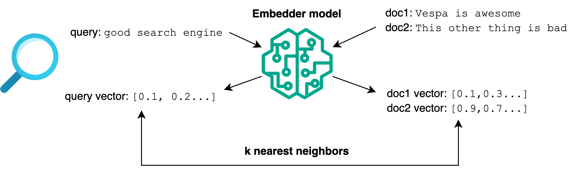
Tensors can also represent embeddings, which can be used for the dense vector search you may already do in Solr. The idea is to get document text through an embedding model and store the result in a tensor field. At query time, we get the query text through the same embedding model and find the closest documents (nearest neighbors).
Here’s an example tensor field definition that stores embeddings:
  field title_embedding type tensor<float>(x[384]) {
    indexing: attribute | index
    attribute {
      distance-metric: angular
    }
  }
Where:
- The tensor will hold 384 float values. For example, representing the embedding of the title.
xis an arbitrary name for our sole dimension. You can have multiple dimensions and multiple tensor fields in a document. We’ll expand on this below.- We enable
attributeto hold the tensor value for computing the ranking. This is needed for both exact kNN and approximate nearest neighbor search (ANN). indexis needed for ANN to build a Hierarchical Navigable Small World (HNSW) graph. Solr also uses HNSW for ANN, but Vespa has one graph per field per node, while Solr has one graph per field per Lucene segment. This accounts for a lot of the performance differences.angularis the distance metric used to compute nearest neighbors. It will effectively order vectors by cosine similarity.
Now you can feed documents with embeddings in them. Alternatively, you can use an embedder to embed the text at write time. This is similar to Solr’s Text-to-Vector, except that it will normally download and run models locally. Many HuggingFace models are supported out of the box, and Vespa use the GPU to generate embeddings.
To use the embedder, you’ll have to define it in your application package under services.xml and then change the schema a bit. For example, the tensor above can change to:
field title_embedding type tensor<float>(x[384]) {
  indexing {
    input title | embed e5_embedder | attribute | index
  }
}
Where title is the field containing the title and e5_embedder is the name of the embedder defined in services.xml. Now you can write documents as they are, and tensors will be automatically populated. Similarly, you can embed the query text at search time and run an ANN search like this:
{
  "yql": "select * from my_document_type where {targetHits:10,approximate:true}nearestNeighbor(title_embedding,query_embedding)",
  "query_text": "hello world query",
  "input.query(query_embedding)": "embed(e5_embedder, @query_text)",
  "ranking.profile": "closeness_rank_profile"
}
Where:
- The nearestNeighbor clause is used to run the ANN search. We know it’s approximate and not exact because we set
approximate:true. targetHitsis the number of documents to return, which might be combined with other query clauses. It’s the equivalent of Solr’stopKin the knn Query Parser.- We look for documents having
title_embeddingclosest toquery_embedding. Which in turn is defined later asinput.query(query_embedding)by embedding the query text (in this case,hello world query, found inquery_text). - Finally, documents are ranked using
closeness_rank_profile. Which can look like this:
  rank-profile closeness_rank_profile {
    inputs {
      # Look for the query_embedding parameter from the query,
      # which should be a 384-dimensional vector, like our title_embedding field
      query(query_embedding) tensor<float>(x[384])
    }
    first-phase {
      # Use the closeness function to rank documents based on
      # the distance-metric defined in the title_embedding field.
      # Here, angular distance (sorting by cosine similarity).
      expression: closeness(field, title_embedding)
    }
  }
Combining vector search with lexical search
Here, we have two use-cases. First, you may want to add filters to your vector search. Something like:
select * from my_document_type where category contains "rock" and nearestNeighbor(title_embedding,query_embedding)
The syntax is quite straightforward, but performance may vary depending on whether you do pre-filtering or post-filtering. Have a look at this blog post for details on how pre- and post-filtering works in Vespa and how you can configure it.
Secondly, you may want to implement hybrid search, where you combine the scores from lexical and vector search. For example, in a query like:
title contains "metallica" or nearestNeighbor(title_embedding,query_embedding)
Then, the magic happens in the rank profile. You can use Reciprocal Rank Fusion (RRF). RRF has to happen in the global phase, where you have access to the global document ranks (i.e., positions in the top N coming from all nodes). Here’s an example RRF implementation:
# we'll reuse the pure vector search rank profile that we defined earlier
rank-profile closeness_rank_profile {
  inputs {
    query(query_embedding) tensor<float>(x[384])
  }
  first-phase {
    expression: closeness(field, title_embedding)
  }
}

# hybrid search rank profile
rank-profile rrf inherits closeness {
  global-phase {
    expression {
      reciprocal_rank_fusion(bm25(title), closeness(field, title_embedding))
    }
    # how many of the top N documents to rerank
    rerank-count: 200
  }
}
Notice how you can use rank profile inheritance to reuse the pure vector search rank profile as if it were a function.
But you’re not limited to RRF. Some people normalize both scores and add them up, maybe with some boosts. Which has two potential advantages:
- Speed, because you can push this normalization down to the second phase, which happens on the content nodes.
- Accuracy, because this method is not lossy like RRF, which only considers document ranks, losing the actual score values.
Below is an example snippet from the multi-vector search sample app. Notice how you can define functions in rank profiles and reuse them:
rank-profile hybrid inherits semantic {
### other functions commented out

    # Lexical score. We can combine these as we see fit.
    function keywords() {
      expression: bm25(title) + bm25(paragraphs) + bm25(url)
    }

    # Normalize the lexical score.
    function log_bm25() {
      expression: if(keywords > 0, log(keywords), 0)
    }

    # Vector search score provides the initial ranking.
    first-phase {
      expression: cos(distance(field,paragraph_embeddings))
    }

    # Then we combine the vector search score with the normalized lexical score.
    second-phase {
      expression {
        firstPhase + log_bm25 + 10*cos(distance(field,paragraph_embeddings))
      }
    }
Since I’ve mentioned multiple vectors per document, let’s have a closer look at how you can definet them in Vespa and why.
Representing multiple vectors per document
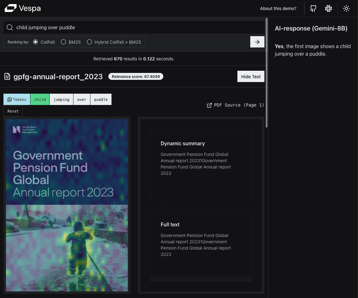
Some models generate multiple vectors per document. For example, ColBERT and ColPali. ColBERT models generate a vector for each token, while ColPali and similar models generate a number of vectors for each image (e.g., a page in a PDF document). Typically, that number is 1024, because it divides the image into 32x32 patches. This allows even highlighting the relevant parts of the image in search results. Here’s a screenshot from our ColPali demo app:
To represent ColPali-generated vectors in Vespa, you can use a tensor field with multiple dimensions. For example:
  document pdf_page {
    field embedding type tensor<float>(patch{}, v[128]) {
      indexing: attribute
    }
  }
Where:
patchis the patch number dimension, one of the 1024 patches in the image.vis the vector dimension. We have just one here.
Solr also supports multiple vectors per document, via block join. But the block join itself adds a performance penalty. By contrast, Vespa will happily have as many dimensions as needed. For example, if a document represents the whole PDF, you can have a page→patch→vector mapping like this:
  document pdf_document {
    field embedding type tensor<float>(page{}, patch{}, v[128]) {
      indexing: attribute
    }
  }
If you want to see a full implementation, have a look at the ColPali demo app on HuggingFace and the corresponding blog resources.
You’ll notice there a different tensor definition compared to those above:
field embedding type tensor<int8>(patch{}, v[16]) {
    indexing: attribute | index
    attribute {
        distance-metric: hamming
    }
That’s because the model they used produces quantized vectors down to one bit per dimension. The type is now an 8-bit integer (a byte) which encodes 8 bits. With 16 such bytes we encode the needed 128 dimensions. To do binary quantization like this, you can either use a model that outputs binary vectors or have Vespa binarize floats for you. Usually, models specifically trained for binary quantization give better results compared to after-the-fact binarization.
Last but not least, for binary vectors, you will want to use hamming distance as the distance metric, which is much faster than other metrics like the angular we used for float vectors.
I hope this gives you a good overview of what you can do with tensors in Vespa. But if your Solr deployment has plugins with custom logic, you might be curious how and if you can translate that to Vespa. Let’s look into Vespa’s hooks next.
Plugin points
Usually, custom logic goes into a container component. These map quite nicely with a lot of Solr plugins:
| Solr plugin | Vespa equivalent | Notes |
|---|---|---|
| Update Request Processors | Document Processors | Both can be chained and modify documents before they are written. |
| Search Components & Query Parsers | Searchers | Like search components, searchers can be chained in a search chain, can parse and modify queries and results. |
| Request Handlers | Request Handlers and Processors | Both can implement custom request-response logic. Processors can be chained. |
| Response Writers | Result Renderers | Both can format the response, e.g. in JSON. |
| Analyzers, Tokenizers, Filters | Linguistics | Both come with default implementations, but you can create your own. |
Conclusion & next steps
Coming from a Solr background, I assume you’ll like:
- Vespa’s tensor support and ranking power. You have even more control than with Solr when it comes to retrieval quality and its performance trade-offs.
- The speeeeeeeeeed 🙂 Especially where tensors are involved: complex ranking, vectors. Even more so if vectors are multi-dimensional.
- The fact that it’s built with production-first in mind: the application packages that you’d normally store in Git, test and deploy with CI/CD, the scaling model that allows you to seamlessly add nodes, etc.
But you might be missing:
- Solr’s dynamic APIs like the schema API and config API. Though if you’re used to putting everything in a configset, the transition to application packages should be smooth.
- The simplicity of running everything in a single JVM process, for small deployments. Vespa Cloud helps here, because it abstracts away the control plane, among other things. And you can easily migrate and scale/autoscale your application to production.
- Solr Admin and other tools from the ecosystem. Vespa’s tooling and community are growing - you might find the IDE support useful, for instance - but we’re not at Solr’s level at the time of this writing.
If you haven’t done this already, I suggest you follow the quickstart tutorials or use Logstash to generate an application package from your data and take it from there. Feel free to reach out on Slack if you get stuck or have any questions!