Scaling ColPali to billions of PDFs with Vespa

This blog post deep dives into scaling “ColPali: Efficient Document Retrieval with Vision Language Models” 1 to large collections of documents. We demonstrate how we can use a phased retrieval and ranking pipeline in Vespa to scale ColPali to billions of documents. To do this, we introduce a new similarity function, a hamming based MaxSim that works with binary vectors produced by binary quantization (BQ). This technique allows us to scale ColPali to large collections of documents while maintaining high accuracy, with a significant reduction in computational cost and vector storage requirements. The suggested deployment also supports real-time indexing and CRUD operation support.
Introduction
ColPali surpasses traditional text-based retrieval methods by leveraging a vision-capable language model, (PaliGemma), to “see” the text, but also the visual elements of a page, including figures, tables and infographics.
ColPali is short for Contextualized Late Interaction over PaliGemma and builds on two key concepts:
-
Contextualized Vision Embeddings from a Vision Language Model (VLM): ColPali generates contextualized embeddings directly from images of pages, using PaliGemma, a powerful VLM with strong visual text understanding capabilities.
-
Late Interaction ColPali uses a late interaction similarity function to compare query and document embeddings at query time, allowing for interaction between all the image grid cell vector representations and all the query text token vector representations.
For a longer introduction to ColPali, see Beyond Text: The Rise of Vision-Driven Document Retrieval for RAG
Do not sleep on VLMs
VLMs have gained popularity for their ability to understand and generate text based on combined text and visual inputs. VLMs display enhanced capabilities in Visual Question Answering (VQA) 2, captioning, and document understanding tasks.
The ColPali model builds on this foundation to tackle the challenge of document retrieval, where the goal is to find relevant documents (pages) based on a user query. The top-k retrieved pages from ColPali could be used for further processing, like summarization or question answering.
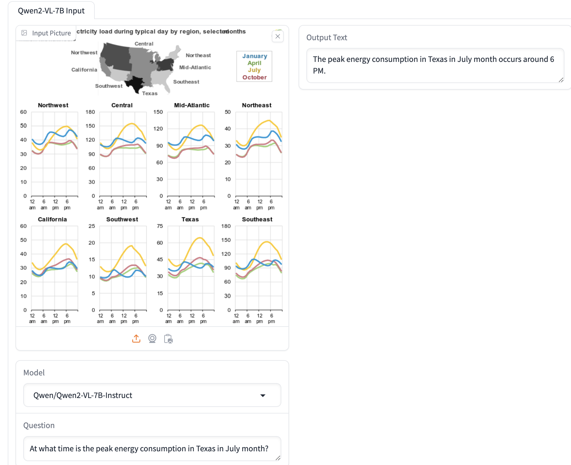 VLM document understanding example. The input to the VLM model is a text question and an image.
The VLM generates an answer (output) based on the question and the image.
This example from a Huggingface Demo Space.
The above illustrates how a VLM can read complex infographics or text rendered in images. The above uses the Qwen/Qwen2-VL-7B-Instruct VLM.
In this example, we provide the VLM with an image of a document page along with a question, and it generates an answer. However, in the context of document retrieval, the goal is to efficiently retrieve the most relevant documents based on a user query, even when working with large collections. Instead of repeating the above process for every page in the collection—which could take days or even years for a single query on a large scale—this approach aims to streamline retrieval and avoid inefficiencies.
Instead, during offline processing of the PDFs, we obtain embeddings for all the pages in the collection, and at query time, run a similarity search over the page embeddings to find the k (e.g. 10) most relevant pages.
This is the approach taken by ColPali and the late interaction similarity mechanism. After having retrieved relevant pages for a query, we can feed the retrieved pages to a VLM for further processing, like summarization or question answering, as demonstrated in the example above.
Scaling VLM retrieval with ColPali
ColPali produces tensors for both the query and the page (technically, the image of a page). The query tensor is made up of text tokens, while the page tensor is made up of image grid cell vectors.
ColPali Page Embeddings: ColPali generates contextualized embeddings solely from images of PDF pages, bypassing the need for text extraction, OCR, and layout analysis. Each image is represented as a 32x32 = 1024 image grid (patches), where each patch is projected into a 128-dimensional latent vector space. In addition to these patch tokens, there is six instruction text tokens that are prepended to the image input: (“Describe the image.”). In total, a single screenshot of a PDF page is represented by 1030 128-d vectors.
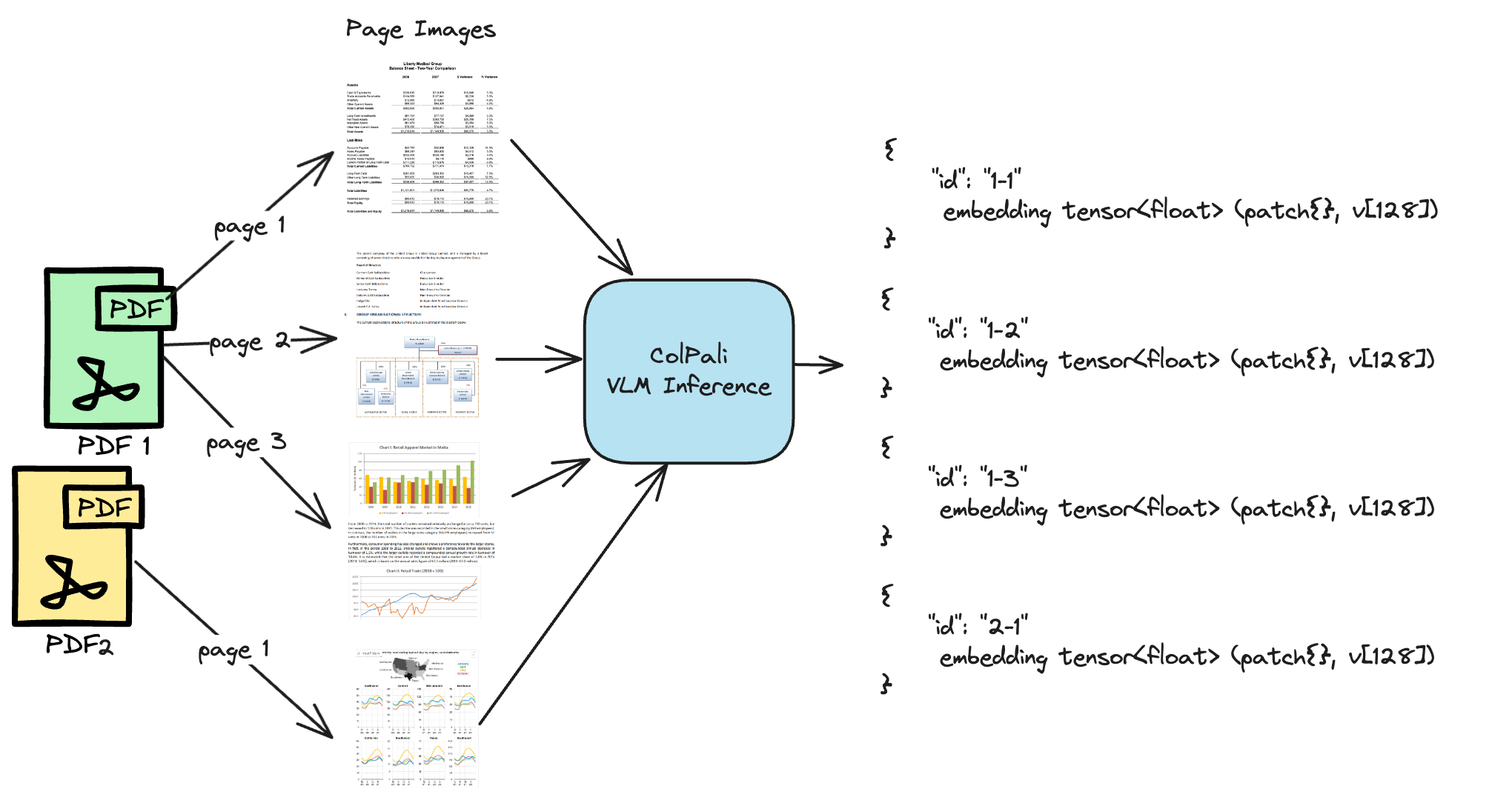
ColPali Query Text Embeddings: The query text is tokenized and each token is also represented in the same latent 128-dimensional vector space as the patch embeddings. The number of query tokens is dynamic (not fixed length as the patch embeddings). The query tokens also include a prefix instruction, “Question: “, and mask padding tokens. This is similar to the query expansion mask tokens used in the ColBERT architecture for the text-only domain.

Using these tensor reprensentation, we can score documents for a query using the late interaction similarity mechanism.
Scoring with MaxSim (The Late Interaction part of ColPali)
ColPali employs a so-called late interaction similarity mechanism, where query and document embeddings are compared at query time using a similarity function, allowing for interaction between all the page patch vector representations and the query text token vector representations.
The late interaction similarity mechanism allows offline embedding generation for all the pages in a collection, and at query time, score and rank the pages based on the similarity between the query and the document embeddings.
Another name for the similarity mechanism used in ColPali is MaxSim, but a more accurate description would be SumMaxSim, as it involves an outer sum operation over the query tokens.
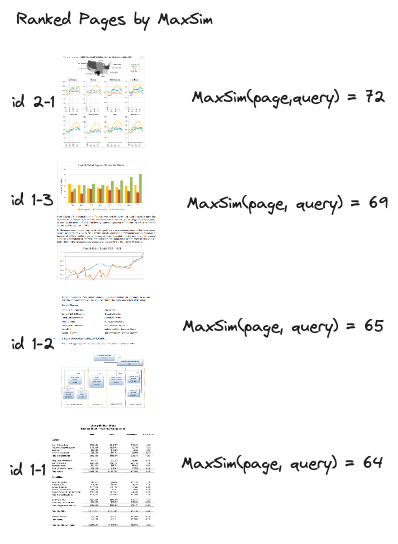
MaxSim ranking of the indexed pages for a query. We want to scale this scoring process to billions of pages.
The MaxSim similarity mechanism is a dot product between all the query token embeddings and all the patch embeddings, followed by a max reduce operation over the patch dimension, followed by a sum reduce operation over the query tokens.
We can represent the tensors and express the MaxSim similarity function using the Vespa schema language.
schema pdf_page {
  document pdf_page {
    field embedding type tensor<float>(p{}, v[128]) {
      indexing: attribute
    }
  }

  model max_sim {
    inputs {
      query(qt) tensor<float>(q{}, v[128])
    }
    function max_sim(query, page) {
      expression {
        sum(
          reduce(
            sum(
              query * page , v
            ),
            max,
            p
          ),
        q
        )
      }
    }
    first-phase {
      expression: max_sim(query(qt), attribute(embedding))
    }
  }
}
Both the embedding field and the input query tensor (query(qt))
are examples of mixed tensors,
combining a named mapped dimension with a named indexed bound dimension (v).
The v dimension is bound and has a fixed size of 128, representing the vector dimension.
The q and p dimensions are unbound and allows representing an unbound number of vectors.
Read more in tensor guide.
Let us zoom in on the MaxSim similarity function:
function max_sim(query, page) {
  expression {
    sum(
      reduce(
        sum(
          query * page , v
        ),
        max,
        p
      ),
      q
    )
  }
}
This function returns a single scalar value representing the MaxSim similarity between the query and the page.
The inner sum of query*page computes the dot product between all the query token embeddings and all the patch embeddings, which results in
a similarity matrix of size [q, p]. We then apply a reduce aggregation over the p dimension using max, and finally
sum over the q dimension.
This function is configured in a the schema in a Vespa ranking expression to rank documents based on the similarity between the query and the document. See a MaxSim example in the Vespa tensor playground.
In PyTorch, a popular deep learning framework, we could express the MaxSim as a function as follows
using the torch.einsum function:
def max_sim(query, page):
  """
  Computes the MaxSim similarity between query and page tensors using einsum.

  Args:
    query: Tensor of shape [querytoken, 128] representing query token vectors.
    page: Tensor of shape [patch, 128] representing page patch vectors.

  Returns:
     the MaxSim similarity score.
  """
  return torch.sum(torch.einsum('qv,pv->qp', query, page).max(dim=1).values, dim=0)
Explanation of the Pytorch max_sim function above:
- torch.einsum(‘qv,pv->qp’, query, page):
Calculates the dot product between
qandpvectors, resulting in a similarity matrix of size[q, p].qvrepresents the query tensor with dimensions querytoken (q) and vector (v).pvrepresents the page tensor with dimensions patch (p) and vector (v).->qpspecifies the output tensor with dimensions querytoken (q) and patch (p).
- .max(dim=1).values:
Finds the maximum value along each row (each query token) of the similarity matrix.
Returns a tensor of size
[q]containing the maximum similarity scores for each query token. - .sum(dim=0): Sums the maximum similarity scores across all query tokens, producing a single scalar value representing the overall MaxSim similarity between the query and the page.
Note that PyTorch does not support unbound dimensions (mapped) or dimension names like Vespa tensors, so we have to specify the dimension sizes.
Scaling MaxSim
MaxSim FLOPs scales with [q * p * v] (roughly). We can reduce the FLOPs
by reducing the number of query tokens (q), the number of patch vectors (p), or the vector dimensionionality (v).
We are interested in scaling a pre-trained model checkpoint and architecture to larger collections of documents, changing
the dimensionality (v) would require retraining the model.
We can reduce the number of patch vector embeddings by pooling or clustering. See the excellent work from Answer.ai on reducing the number of document vectors in their blog post: A little pooling goes a long way for multi-vector representations.
Another direction is to use a cheaper similarity function than dot product, in other words, a function that requires fewer CPU instructions than float dot products. This can also be used in combination with pooling or clustering to reduce the number of vectors to score.
An alternative to a float dot product is the inverted hamming distance, which is a simple and fast distance function. The hamming distance is the number of positions at which the corresponding bits are different, and can be computed with fewer CPU instructions than a float dot product.
To use hamming distance in Vespa, we need to represent the ColPali text and patch vectors as binary vectors,
using the int8 tensor cell type in Vespa, where we can
“pack” the 128-dim float vectors into 16-dim int8 tensors in Vespa. Each int8 cell represents 8 bits.
The following demonstrates how we can use the hamming
distance instead of float dot product as the core similarity in MaxSim.
Since hamming
is a distance metric (closer to 0 is more similar), we invert the distance to a similarity score by inversion: 1/(1 + hamming(query, page)).
(Note that hamming is a built in Vespa ranking expression function):
schema pdf_page {
  document pdf_page {
    field embedding type tensor<int8>(p{}, v[16]) {
      indexing: attribute
    }
  }

  model max_sim {
    inputs {
      query(qt) tensor<int8>(q{}, v[16])
    }
    function max_sim(query, page) {
      expression {
        sum(
          reduce(
            1/(1 + sum(
              hamming(query, page) ,v)
            ),
            max,
            p
          ),
          q
        )
      }
    }

    first-phase {
      expression: max_sim(query(qt), attribute(embedding))
    }
  }
}
We use binary quantization (BQ) to convert the floating point 128-dimensional vectors to 128-bit vectors, represented in the schema as 16-d vector with cell type int8. See our blog post on Matryoshka 🤝 Binary vectors: Slash vector search costs with Vespa for more information about hamming distance and binary quantization.
With this approach, we can reduce the number of CPU instructions required to compute the similarity between the query and the document, making the MaxSim ranking process more efficient.
Optimizing the MaxSim with hamming
In this Vespa performance test, we measure and track the difference in latency between the two versions of the MaxSim function.
This test simulates ranking 1,000 pages for a query with 20 vectors and 1030 vectors per page, using a single CPU core. It’s important to notice that we can scale latency linearly (almost) with the number of CPU cores by Vespa intra-query multi-threading.
In the performance test we measure the end-to-end latency of the two MaxSim versions. With a single ranking thread, latency is a good proxy for computional cost.
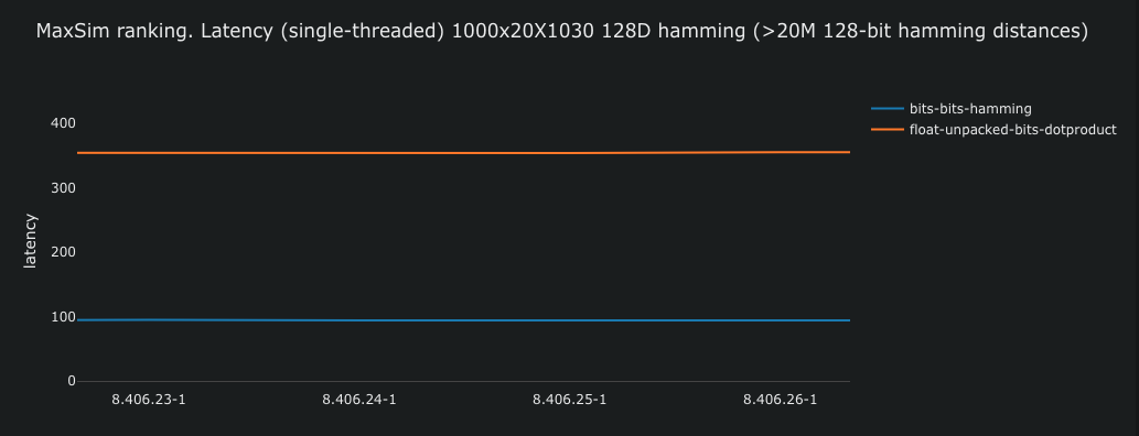
The blue line represents the hamming distance version of the MaxSim function, while the orange line represents the float dot product version. As we can see the hamming version is about 3.5 times faster than the float dot product version. This means that we can rank more pages for the same latency budget or lower the latency for the user query. For services that doesn’t nessessarily need high query throughput, but were we want to lower latency for a better user experience, we can throw CPU cores at the problem using intra-query multithreading to reduce latency further, e.g by using 2 or 4 CPU cores we can reduce latency by a factor of 2 or 4, respectively.
With 1000 pages, 20 query token vectors, and 1030 patch vectors, the MaxSim involves 20M 128-dimensions dot products or 128-dimensions hamming distances (bitwise). For the hamming version, with 100ms latency, this translates to about 200M 128-bit hamming distances per second per CPU core/thread.
As part of this work with scaling ColPali, we optimized
the evaluation of the 1/(1 + sum(hamming(query, page), v)) expression. This is done by recognizing the specific use case,
allowing for HW optimized evaluation by the Vespa tensor engine. This
type of optimization was already in place for the float dot product version after our work with ColBERT.
Scaling to Billions of Documents
So far we have discussed how to compute the MaxSim similarity function without considering the scale of the document collection. Performing MaxSim over 1000 pages in an index is not a huge problem. We can brute-force score and rank all of them for every query.
But at larger scale (either #documents or #queries), we need to distribute the computation across multiple nodes and also find a way to perform candidate selection (retrieval) so that we avoid scoring all the pages (brute-force) with the MaxSim expression. This is where Vespa’s phased retrieval and ranking pipeline comes into play.
The standard retrieval strategy for ColBERT and ColPali is to use approximate nearestNeighbor search to retrieve candidate documents based on the query token embeddings, and then rank the retrieved documents using MaxSim.
For example, if we have 20 query token vectors, we do a candidate search for each of the 20 query token vectors and the union
of the candidate sets are ranked using MaxSim. Each nearest neighbor operation finds the closest k pages with the closest
patch vector to the query token vector.
Vespa supports multi-vector HNSW indexing, so we can index multiple patch vectors per page, and perform approximate nearest neighbor search over all the patch vectors in a single query.
field embedding type tensor<int8>(p{}, v[16]) {
  indexing: attribute | index
  attribute {
    distance-metric: hamming
  }
  index {
    hnsw {
      max-links-per-node: 32
      neighbors-to-explore-at-insert: 200
    }
  }
}
We use the hamming distance metric
for this index. We enable HNSW by adding index
to the embedding field in the schema. Notice also how we configure the distance-metric and HNSW index hyper parameters
that are tradoffs between speed and accuracy (comparing to exact nearest neighbor search).
For a single query token vector we could do a nearest neighbor search over all the patch vectors using the Vespa nearestNeighbor query operator using the Vespa query language:
{
  "yql": "select documentid, embedding from pdf_page where {targetHits:100}nearestNeighbor(embedding,q1)",
  "input.query(q1)": [23,-34,12,45,67,23,45,12,45,67,23,45,12,45,67,23],
  "ranking": "vector_similarity_only",
  "hits": 100
}
This query would return the 100 closest pages to the query token vector q1 based on the hamming distance to the closest patch vector in the page.
However, we do not want to run one nearest neighbor query for each query token vector, but rather run a single Vespa query that exposes the top-k pages for all the query token vectors to a Vespa ranking expression. This allows scoring and ranking using MaxSim without transferring the page vectors to some external ranking service.
Why? Consider the case where we have 20 query token vectors, and where we want to retrieve the top-100 pages for each query token vector for MaxSim re-ranking, we would have up to 2K (20x100) pages to rank using a MaxSim implementation. Each page is made up of 1030 vectors with 16 bytes (int8 values), each user query request would need to transfer 2K x 1030 x 16 bytes ±= 32MB of data to the “MaxSim ranking service”. This is sequential latency added before we start scoring the pages with MaxSim.
At any meaningful query throughput scale, fetching this amount of vector data per user query would quickly become a scaling bottleneck even with a fast high-throughput network.
Instead, we want to move the tensor computations (here MaxSim) to the data and instead perform the candidate selection and ranking in a single Vespa query request using multiple nearest neighbor operators, combined using boolean operators (which also allows combining ColPali/ColBERT with query filters).
{
  "yql": "select documentid from pdf_page where ({targetHits:100}nearestNeighbor(embedding,q1)) or ({targetHits:100}nearestNeighbor(embedding,q2))",
  "input.query(q1)": [23,-34,12,45,67,23,45,12,45,67,23,45,12,45,67,23],
  "input.query(q2)": [12,4,87,23,45,12,45,67,23,45,12,45,67,23,45,12],
  ....
  "ranking": "max_sim",
  "hits": 10
}
A Vespa schema for scalable retrieval and ranking of ColPali could look like this, note that all the input query tensors are
defined
in the model section of the schema (model is also an alias for rank-profile). We can define as many
input query tensors as we want or need. Defining query tensors
has no overhead, as the input tensors are only used when a query is executed.
schema pdf_page {
  document pdf_page {
    field embedding type tensor<int8>(p{}, v[16]) {
      indexing: attribute | index
      attribute {
        distance-metric: hamming
      }
      index {
        hnsw {
          max-links-per-node: 32
          neighbors-to-explore-at-insert: 200
        }
      }
    }
  }

  model max_sim {
    inputs {
      query(qt) tensor<int8>(q{}, v[16])
      query(q1) tensor<int8>(v[16])
      query(q2) tensor<int8>(v[16])
      query(q3) tensor<int8>(v[16])
      query(q4) tensor<int8>(v[16])
      ....
    }
    function max_sim(query, page) {
      expression {
        sum(
          reduce(
            1/(1 + sum(
              hamming(query, page) ,v)
            ),
            max,
            p
          ),
          q
        )
      }
    }
    first-phase {
      expression: max_sim(query(qt), attribute(embedding))
    }
  }
}
With this type of schema, we can perform a query request where we both retrieve candidate documents and rank them in a single request as the nearestNeighbor query operator in Vespa can be combined using boolean operators and combined with filters.
This type of retrieval and ranking pipeline for late-interaction models avoids the need to transfer large amounts of vector data between services as everything is computed inside the Vespa content nodes. Inside the content node, we can transfer vector data at the speed of memory and not the network. This is a core design principle in Vespa, allowing developers to express complex ranking pipelines that might involve lots of vector data in a single query request.
Note that with the query tensor separation, where there are N single-vector representing each query token vector and a single mixed
tensor used for the MaxSim ranking, we can also perform query token pruning 3 4. By using a subset of the query token vectors
we can speed up the retrieval phase, and rank fewer pages with the MaxSim variants. Pruning attempts to
remove less important query token vectors from the retrieval phase while they are retained for the ranking phase.
This query tensor separation also allows different levels of targetHits per query token vector
for the retrieval phase.
Is hamming a good similarity function for ColPali?
In the previous sections, we discussed how to scale ColPali to billions of documents using Vespa’s phased retrieval and ranking pipeline, using hamming distance for the nearest neighbor search and MaxSim for ranking. How does this approach perform in practice?
We evaluated the performance of the ColPali model on the DocVQA dataset using the ColPali embeddings and the proposed hamming-based MaxSim function in Vespa.
In the following we compare four different ranking strategies on the DocVQA test dataset using nDCG@5 as the evaluation metric. The four strategies are:
- float-float The “normal” float dot product in MaxSim
- binary-binary The suggested hamming-based MaxSim
- binary-binary-reranking Adding a re-ranking phase on top of the binary-binary version. In the re-ranking phase we are using float resolution for the query tensor, but an unpacked float representation obtained from the binary vector. This step requires that we pass both the representations of the query tensor to Vespa.
| float-float | 52.4 |
| binary-binary (hamming) | 49.5 |
| binary-binary (hamming) + float-float re-ranking | 51.6 |
A notebook that demonstrates the impact of re-ranking depth can be found here. As seen from the above table, we can save 32x on storage (memory) by using the binary representation instead of float, make MaxSim 4x more efficient by using hamming distance, and retain the most of the accuracy. The drop from 52.4 to 51.6 is a small price to pay for the efficiency gain.
Summary
ColPali is a groundbreaking document retrieval model, probably one of the most significant advancements in the field of document retrieval in recent years. By leveraging the power of vision language models, ColPali can effectively retrieve documents based on both textual and visual information in them. With the increased interest in scaling ColPali to large collections of PDF documents, Vespa provides a powerful platform for implementing and deploying ColPali at scale.
ColPali or VLMs in general simplifies the ingestion pipeline by eliminating the need for text extraction, OCR, and layout analysis. This makes it easier to implement and deploy in real-world applications with fewer preprocessing and extraction steps.
As part of this blog, we have also created a comprehensive notebook that demonstrates all the concepts discussed in this blog post, check it out here: Scaling ColPali with Vespa.
The demo notebook features:
- Obtaining ColPali embeddings for queries and PDF pages
- How to use the MaxSim similarity function in Vespa and use both versions in a phased ranking pipeline
- How to use the Vespa nearestNeighbor query operator to retrieve candidate documents for ranking
In addition, we also demonstrate how to reproduce the accuracy results on the DocVQA dataset using the ColPali embeddings and the MaxSim similarity functions described in this post: ColPali Benchmark DocVQA.
If you want to learn more about ColPali, and how to represent ColPali in Vespa, also check our previous posts on ColPali and Vespa.
- Beyond Text: The Rise of Vision-Driven Document Retrieval for RAG
- PDF Retrieval with Vision Language Models
Other useful resources on ColPali:
- Notebook Scaling ColPali with Vespa
- Notebook Complex ColPali + Vespa
- ColPali Paper
- ColPali on GitHub
For those interested in learning more about Vespa or ColPali, feel free to join the Vespa community on Slack or Discord to exchange ideas, seek assistance from the community, or stay in the loop on the latest Vespa developments. Also check out the FAQ section below for more information on how to use ColPali in Vespa.
FAQ
Why can’t you just use a frontier like VLM with a large context window for this?
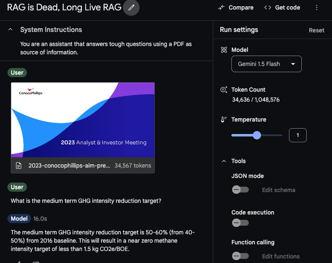 Screenshot from Google AI studio using Gemini FLash with a large context window for RAG.
Frontier VLM models like GPT-4/Gemini Flash handles visual inputs well (The PDF above is converted to images of the PDF pages, just like ColPali), but they have a limited context window.
In this case, a 62-page PDF occupies 34,567 tokens so that we can fit about 30 of those into the LLM context window.
We argue that there are use cases where you want to retrieve over more extensive collections than 30.
In addition, as can be seen above, inference takes about 16 seconds for every query over this single PDF.
Certainly, foundational models with large context windows can be used for RAG over small collections, but with high latency. They are not a universal solution for large collections of complex document formats.
In this case, you turn to ColPali to retrieve relevant pages, and then feed those to the foundational model to generate the best of two paradigms.
I have many structured text fields and meta data, can I use ColPali in Vespa?
Yes, you can combine the ColPali embeddings with other features in Vespa.
Can I combine ColPali with query filters in Vespa?
Yes, ColPali, is primarily a way to score documents based on a query, and can be combined with any Vespa query formulation, including filters, and also result grouping.
Our custom ranking uses many business-oriented ranking signals, can I use ColPali?
Yes, Vespa’s ranking framework allows many different signals of rank features as we call them in Vespa. Features can be combined in ranking expressions in ranking phases.
The MaxSim expression can be used as any other feature, and in combination with other custom features, even as a feature in a GBDT-based ranker using Vespa’s xgboost or lightgbm support.
How does ColPali relate to Vespa’s support for nearestNeighbor search? If we want to use ColPali representations in retrieval and not just for ranking, we can use the Vespa nearestNeighbor search operator to retrieve candidate documents based on the query token embeddings. The candidate documents are then ranked using the MaxSim similarity function (and or custom ranking features) in a Vespa ranking expression.
How does ColPali relate to Vespa HNSW indexing for mixed tensors or multi-vectors? It’s handy if we need to use ColPali representations for retrieval, allowing for efficient candidate selection based on the query token embeddings. See more in multi-vector indexing.
Any plans to integrate ColPali as a native Vespa embedder
Yes, see this issue.
Can I combine ColPali with ColBERT in Vespa? Yes, you can combine ColPali with ColBERT or SPLADE or other fancier text ranking method in Vespa. Those would be two different embedding (tensor) fields in the Vespa schema, and you can use two (or multiple) MaxSim expressions and combine the score in ranking expressions.
How does ColPali compare to hybrid search?
ColPali can be used in a hybrid search
pipeline
as just another neural scoring feature, used in any of the Vespa
ranking phases (preferably in second-phase for optimal performance
to avoid moving vector data up the stateless container for
global-phase evaluation).
Vespa allows combining the MaxSim score with other scores using, for example, reciprocal rank fusion or other normalization rank features. The sample application features examples of using ColBERT MaxSim in a hybrid ranking pipeline.
Can I run ColPali if I’m GPU-poor?
Yes, you can. All the notebooks were developed using PyTorch with MPS support on M1 Macs, and the Vespa content backend is CPU-based.
Encoding the PDF pages takes about 2.5 seconds per page with batches of 4 on MPS (if you ensure to close down Chrome or other GPU-hungry applications). PaliGemma works well with batch size 4 on a 16GB T4 GPU (or similar).
What are the tradeoffs? If it stores a vector per patch, it must be expensive!
We can look at performance and deployment cost along three axes: Effectiveness (ranking quality), storage, and computations. In this context, we can recommend Moving Beyond Downstream Task Accuracy for Information Retrieval Benchmarking, which provides a framework to compare different methods.
A natural comparision is recent large decoder-based text embedding models (e.g. NV-Embed-v2) that produces 4096-dimensional float embeddings for short texts, their storage footprint is 16KB per chunk (and you will need more than one chunk to accurately represent a page). ColPali with binarized patch vectors has a similar storage footprint (16KB).
In practise, this means that ColPali is more storage efficient than large decoder-based text embedding models, but requires more computations to score and rank the documents (as we have to compute the MaxSim similarity function).
Why didn’t you expose the ColBERT 2 PLAID retrieval optimization in Vespa? Could this be an alternative for scaling ColPali?
Primarily because Vespa is designed for low-latency real-time indexing with CRUD support. The PLAID indexing optimization requires batch processing the document token vectors to find centroids. This centroid selection would not scale in a real-time setting where users expect outstanding performance from document number one to billions of documents. As demonstrated in this post, we can replace the float dot product with a hamming distance, which is a much faster operation than a float dot product and then we can use the Vespa nearestNeighbor query operator to retrieve candidate documents for ranking. This makes the approach more scalable and efficient for real-time document retrieval.
That is a lot of hamming distances - do you use any acceleration to speed it up?
Yes, Vespa’s core backend is written in C++, and the dot products and hamming are accelerated
using SIMD instructions.
Is ColPali good or not? ColPali is a more of a direction than a model checkpoint to rule them all. We believe in the power of vision language models for complex document retrieval, and we are excited to see how the field evolves. We envision a future where we can have models trained on different VLM backbones like Qwen/Qwen2-VL-7B-Instruct.
Can I use ColPali for other tasks than document retrieval? The ColPali model is actually a Low-Rank Adapter (LoRA) model on top of PaliGemma, so you can use it for any task that PaliGemma is good at if you remove the adapter layer.
References
-
ColPali: Efficient Document Retrieval with Vision Language Models ↩
-
MMLongBench-Doc: Benchmarking Long-context Document Understanding with Visualizations ↩
-
Query Embedding Pruning for Dense Retrieval , Nicola Tonellotto, Craig Macdonald ↩
-
An Analysis on Matching Mechanisms and Token Pruning for Late-interaction Models ↩
