In this blog post we’ll explain how to use Vespa to evaluate TensorFlow models over arbitrarily many data points while keeping total latency constant. We provide benchmark data from our performance lab where we compare evaluation using TensorFlow serving with evaluating TensorFlow models in Vespa.

We recently introduced a new feature that enables direct import of TensorFlow models into Vespa for use at serving time. As mentioned in a previous blog post, our approach to support TensorFlow is to extract the computational graph and parameters of the TensorFlow model and convert it to Vespa’s tensor primitives. We chose this approach over attempting to integrate our backend with the TensorFlow runtime. There were a few reasons for this. One was that we would like to support other frameworks than TensorFlow. For instance, our next target is to support ONNX. Another was that we would like to avoid the inevitable overhead of such an integration, both on performance and code maintenance. Of course, this means a lot of optimization work on our side to make this as efficient as possible, but we do believe it is a better long term solution.

Naturally, we thought it would be interesting to set up some sort of performance comparison between Vespa and TensorFlow for cases that use a machine learning ranking model.

Before we get to that however, it is worth noting that Vespa and TensorFlow serving has an important conceptual difference. With TensorFlow you are typically interested in evaluating a model for a single data point, be that an image for an image classifier, or a sentence for a semantic representation etc. The use case for Vespa is when you need to evaluate the model over many data points. Examples are finding the best document given a text, or images similar to a given image, or computing a stream of recommendations for a user.

So, let’s explore this by setting up a typical search application in Vespa. We’ve based the application in this post on the Vespa blog recommendation tutorial part 3. In this application we’ve trained a collaborative filtering model which computes an interest vector for each existing user (which we refer to as the user profile) and a content vector for each blog post. In collaborative filtering these vectors are commonly referred to as latent factors. The application takes a user id as the query, retrieves the corresponding user profile, and searches for the blog posts that best match the user profile. The match is computed by a simple dot-product between the latent factor vectors. This is used as the first phase ranking. We’ve chosen vectors of length 128.

In addition, we’ve trained a neural network in TensorFlow to serve as the second-phase ranking. The user vector and blog post vector are concatenated and represents the input (of size 256) to the neural network. The network is fully connected with 2 hidden layers of size 512 and 128 respectively, and the network has a single output value representing the probability that the user would like the blog post.

In the following we set up two cases we would like to compare. The first is where the imported neural network is evaluated on the content node using Vespa’s native tensors. In the other we run TensorFlow directly on the stateless container node in the Vespa 2-tier architecture. In this case, the additional data required to evaluate the TensorFlow model must be passed back from the content node(s) to the container node. We use Vespa’s fbench utility to stress the system under fairly heavy load.

In this first test, we set up the system on a single host. This means the container and content nodes are running on the same host. We set up fbench so it uses 64 clients in parallel to query this system as fast as possible. 1000 documents per query are evaluated in the first phase and the top 200 documents are evaluated in the second phase. In the following, latency is measured in ms at the 95th percentile and QPS is the actual query rate in queries per second:

• Baseline: 19.68 ms / 3251.80 QPS
• Baseline with additional data: 24.20 ms / 2644.74 QPS
• Vespa ranking: 42.8 ms / 1495.02 QPS
• TensorFlow batch ranking: 42.67 ms / 1499.80 QPS
• TensorFlow single ranking: 103.23 ms / 619.97 QPS

Some explanation is in order. The baseline here is the first phase ranking only without returning the additional data required for full ranking. The baseline with additional data is the same but returns the data required for ranking. Vespa ranking evaluates the model on the content backend. Both TensorFlow tests evaluate the model after content has been sent to the container. The difference is that batch ranking evaluates the model in one pass by batching the 200 documents together in a larger matrix, while single evaluates the model once per document, i.e. 200 evaluations. The reason why we test this is that Vespa evaluates the model once per document to be able to evaluate during matching, so in terms of efficiency this is a fairer comparison.

We see in the numbers above for this application that Vespa ranking and TensorFlow batch ranking achieve similar performance. This means that the gains in ranking batch-wise is offset by the cost of transferring data to TensorFlow. This isn’t entirely a fair comparison however, as the model evaluation architecture of Vespa and TensorFlow differ significantly. For instance, we measure that TensorFlow has a much lower degree of cache misses. One reason is that batch-ranking necessitates a more contiguous data layout. In contrast, relevant document data can be spread out over the entire available memory on the Vespa content nodes.

Another significant reason is that Vespa currently uses double floating point precision in ranking and in tensors. In the above TensorFlow model we have used floats, resulting in half the required memory bandwidth. We are considering making the floating point precision in Vespa configurable to improve evaluation speed for cases where full precision is not necessary, such as in most machine learned models.

So we still have some work to do in optimizing our tensor evaluation pipeline, but we are pleased with our results so far. Now, the performance of the model evaluation itself is only a part of the system-wide performance. In order to rank with TensorFlow, we need to move data to the host running TensorFlow. This is not free, so let’s delve a bit deeper into this cost.

The locality of data in relation to where the ranking computation takes place is an important aspect and indeed a core design point of Vespa. If your data is too large to fit on a single machine, or you want to evaluate your model on more data points faster than is possible on a single machine, you need to split your data over multiple nodes. Let’s assume that documents are distributed randomly across all content nodes, which is a very reasonable thing to do. Now, when you need to find the globally top-N documents for a given query, you first need to find the set of candidate documents that match the query. In general, if ranking is done on some other node than where the content is, all the data required for the computation obviously needs to be transferred there. Usually, the candidate set can be large so this incurs a significant cost in network activity, particularly as the number of content nodes increase. This approach can become infeasible quite quickly.

This is why a core design aspect of Vespa is to evaluate models where the content is stored.

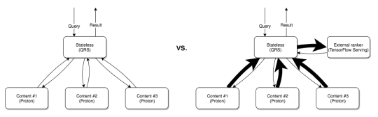
This is illustrated in the figure above. The problem of transferring data for ranking is compounded as the number of content nodes increase, because to find the global top-N documents, the top-K documents of each content node need to be passed to the external ranker. This means that, if we have C content nodes, we need to transfer C*K documents over the network. This runs into hard network limits as the number of documents and data size for each document increases.

Let’s see the effect of this when we change the setup of the same application to run on three content nodes and a single stateless container which runs TensorFlow. In the following graph we plot the 95th percentile latency as we increase the number of parallel requests (clients) from 1 to 30:

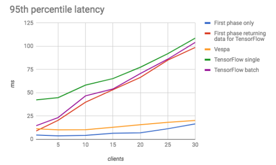
Here we see that with low traffic, TensorFlow and Vespa are comparable in terms of latency. When we increase the load however, the cost of transmitting the data is the driver for the increase in latency for TensorFlow, as seen in the red line in the graph. The differences between batch and single mode TensorFlow evaluation become smaller as the system as a whole becomes largely network-bound. In contrast, the Vespa application scales much better.

Now, as we increase traffic even further, will the Vespa solution likewise become network-bound? In the following graph we plot the sustained requests per second as we increase clients to 200:

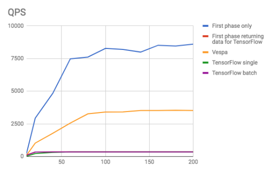
Vespa ranking is unable to sustain the same amount of QPS as just transmitting the data (the blue line), which is a hint that the system has become CPU-bound on the evaluation of the model on Vespa. While Vespa can sustain around 3500 QPS, the TensorFlow solution maxes out at 350 QPS which is reached quite early as we increase traffic. As the system is unable to transmit data fast enough, the latency naturally has to increase which is the cause for the linearity in the latency graph above. At 200 clients the average latency of the TensorFlow solution is around 600 ms, while Vespa is around 60 ms.

So, the obvious key takeaway here is that from a scalability point of view it is beneficial to avoid sending data around for evaluation. That is both a key design point of Vespa, but also for why we implemented TensorFlow support in the first case. By running the models where the content is allows for better utilization of resources, but perhaps the more interesting aspect is the ability to run more complex or deeper models while still being able to scale the system.