
We announce support for combining matryoshka and binary quantization in Vespa’s native hugging-face embedder (Vespa >= 8.332.5). In addition, we discuss how these techniques slash costs compared to float text embeddings.
Recent advances in text embedding models include matryoshka representation learning(MRL), which creates a hierarchy of embeddings with flexible dimensionalities, and binary quantization learning (BQL), which learns to encode float dimensions to 1-bit representation, representing text as a binary vector.
Both MRL and BQL are instances of deep representational learning, albeit with variations in their representations.
 Instead of representing text as a large vector of floats, the combination of MRL and BQL encodes text
as a binary vector, no longer than a SHA-512 hash (512 bits).
Instead of representing text as a large vector of floats, the combination of MRL and BQL encodes text
as a binary vector, no longer than a SHA-512 hash (512 bits).
The emphasis of both MRL and BQL is on sacrificing accuracy by a few % in exchange for a much lower cost. By using a compact representation of the text embeddings, the systems can run on less expensive hardware or require less memory, resulting in cost savings. We can quantify the memory-related savings using Vespa basic plan pricing, where memory (GB) is priced at $ 0.01 / hour. In the following table, we calculate the memory price for 1 Billion 1024-dimensional vectors using different Vespa tensor precision types.
| Vector precision | Vector dimensions | Bytes per vector | GB for 1B vectors | $ hourly |
| float | 1024 | 4096 | 3814 | 38.14 |
| bfloat16 | 1024 | 2048 | 1907 | 19.07 |
| int8 (scalar quantization) | 1024 | 1024 | 953 | 9.54 |
| int8 (binary quantization) | 128 | 128 | 119 | 1.19 |
| int8 (binary quantization + mrl) | 64 | 64 | 60 | 0.59 |
Assuming the use case is within Vespa’s vector streaming search capabilities, which is suitable for scenarios with partitioned data (e.g., by user ID) and disk-based storage, we can significantly reduce the hourly pricing. In such cases, the $0.01/hour cost can be reduced to $0.0004/hour, effectively reducing the above hourly prices by 25. Moreover, similarity searches over these binary representations are fast in Vespa, which slashes the CPU-related costs, demonstrated in later sections.
In addition to cost savings for existing use cases, MRL and BQL will unlock new ones that are no longer prohibitively costly when vector size drops much below the original text size. This binary text embedding paradigm shift will make more unstructured data useful with binary embedding representations.
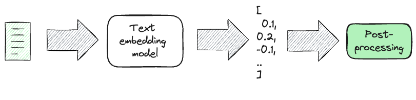
Since both techniques are simple post-processing steps over the embedding vector representation, we can produce multiple representations with a single model inference call. One inference pass is vital because model inference is a significant cost driver for embedding retrieval systems.
For MRL, the post-processing stage retains the first k dimensions
of the original n dimensions; in contrast, binary quantization retains the
dimensionality but converts the float dimension values into a 1-bit
representation via thresholding normalized embeddings at 0.
- MRL provides flexibility in the number of dimensions
- BQL provides per-dimension precision flexibility
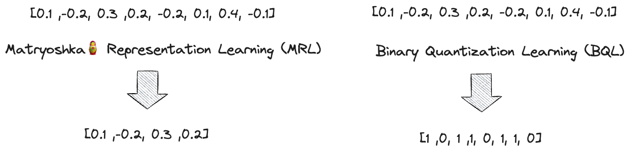 MRL retains only the first k-dimensions of the original vector representation, while BLQ learns
a binary representation.
MRL retains only the first k-dimensions of the original vector representation, while BLQ learns
a binary representation.
An exciting new direction in embedding models is to combine these two techniques. From Binary and Scalar Embedding Quantization for Significantly Faster & Cheaper Retrieval:
Additionally, we are excited that embedding quantization is fully perpendicular to Matryoshka Representation Learning (MRL). In other words, it is possible to shrink MRL embeddings from e.g. 1024 to 128 (which usually corresponds with a 2% reduction in performance) and then apply binary or scalar quantization.
This turned out to be a solid direction, as demonstrated by mixedbread.ai in their follow-up blog post: 64 bytes per embedding, yee-haw.
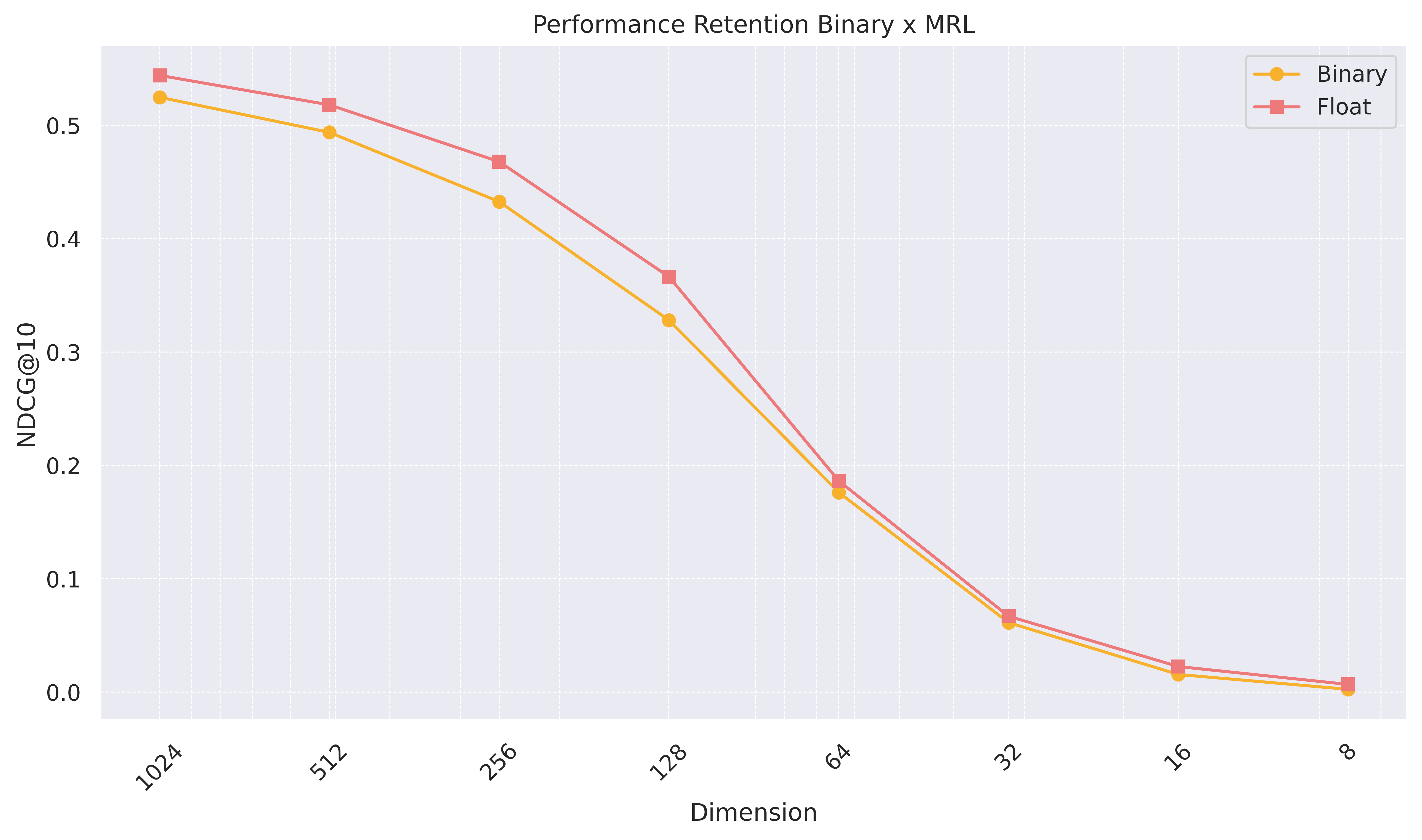 Illustration from mixedbread.ai blog post. Notice the small gap between
the binary representation and the float representation. At 512 dimensions, the binary representation is 64 bytes.
Illustration from mixedbread.ai blog post. Notice the small gap between
the binary representation and the float representation. At 512 dimensions, the binary representation is 64 bytes.
Mixedbread.ai’s combination of MRL and BQL retains 90% accuracy (on
MTEB Retrieval task) using 64-dimensional int8 (512 bits)
binarized from 512 float dimensions (first 512 out of 1024).
This binary representation reduces storage-related costs by 64
compared to the baseline using 1024 floats.
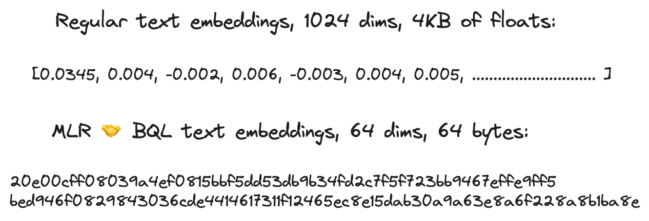
Notably, the text embedding storage requirement drops to 64 bytes per vector embedding; the same size as a SHA-512 hash:
20e00cff08039a4ef0815bbf5dd53db9b34fd2c7f5f723bb9467effe9ff5
bed946f0829843036cde4414617311f12465ec8e15dab30a9a63e8a6f228a8b1ba8e
Hex representation of a 64-dimensional int8 vector, 128 characters. Illustration of how compact state-of-the-art text binary embeddings are. Vespa supports hex format of binary vectors in both queries and in documents. Compare this compact representation with wrestling with thousands of float dimensions..
Adapting MRL and BQL with embedding inference in Vespa
Vespa exposes core functionality for embedding text to vector representations, in queries and documents. This functionality allows developers to embed (pun intended) their chosen text embedding models in Vespa, scale inference volume, and reduce query latency by avoiding sending large vector payloads over remote networks. As a bonus, it eliminates wrestling with additional infrastructure for embedding inference.
With the increased interest in MRL and BQL we have added support for obtaining MRL and BQL embeddings to the native Vespa hugging-face-embedder.
We demonstrate the new functionality using mixedbread.ai’s text embedding model which has been trained with both a MRL and BQL objective. The mixedbread.ai embedding model has 1024 float dimensions originally, but offers dimension flexibility via MRL and precision flexibility via BQL. The mixedbread.ai model uses CLS pooling, and the float version uses the prenormalized-angular distance metric where vectors are normalized to unit length (1) and where the cosine similarity equals the dot product between two vectors. For the binarized version, hamming distance is used as distance-metric. See the adaptive retrieval section for more details on these two distance metrics.
First, we add the component of type hugging-face-embedder to the Vespa application package services.xml,. Notice pooling-strategy and normalization.
<component id="mxbai" type="hugging-face-embedder">
  <transformer-model url="https://huggingface.co/mixedbread-ai/mxbai-embed-large-v1/resolve/main/onnx/model_fp16.onnx"/>
  <tokenizer-model url="https://huggingface.co/mixedbread-ai/mxbai-embed-large-v1/raw/main/tokenizer.json"/>
  <pooling-strategy>cls</pooling-strategy>
  <normalize>true</normalize>
 </component>
For GPU instances in Vespa Cloud, we recommend the fp16 model for 3x throughput over the standard model (fp32). For CPU instances, use the quantized model version.
The following demonstrates the new functionality for embedding texts using the Vespa hugging-face-embedder. All the schema examples below use a single text field. The embed functionality can also handle arrays of strings with multi-vector indexing support.
schema doc {
  document doc {
  	field text type string {..}
  }
  field embedding type tensor<float>(x[1024]) {
     indexing: input text | embed mxbai | attribute | index
     attribute {
        distance-metric: prenormalized-angular
     }
  }
}
In the example above, we retain the full precision representation
(1024 floats), signaled by having a destination tensor type
tensor<float>(x[1024]. The index is optional and will build
a HNSW graph
for the tensor. HNSW index enables efficient but approximate nearest neighbor
search.
If we want to use the first 256 dimensions instead (MRL), we can
signal that by changing the tensor definition from x[1024] to x[256]
and the embedder will use the first 256 dimensions of the model’s original output
dimensions.
schema doc {
  document doc {
  	field text type string {..}
  }
  field mrl_embedding type tensor<float>(x[256]) {
     indexing: input text | embed mxbai | attribute | index
     attribute {
        distance-metric: prenormalized-angular
     }
  }
}
We can also change the tensor cell
type to
bfloat16 instead of float, which reduces storage by 2x over
float (but is computationally approximately 20% slower than float
on CPU).
field mrl_embedding type tensor<bfloat16>(x[256]) {
     indexing: input text | embed mxbai | attribute | index
     attribute {
        distance-metric: prenormalized-angular
     }
}
We can also obtain multiple representations. The schema below will only involve a single inference call to the model because it uses the same input text and the same embedder id.
schema doc {
  document doc {
  	field text type string {..}
  }

  field mrl_embedding type tensor<bfloat16>(x[256]) {
     indexing: input text | embed mxbai | attribute | index
     attribute {
        distance-metric: prenormalized-angular
     }
  }

  field embedding type tensor<bfloat16>(x[1024]) {
     indexing: input text | embed mxbai | attribute
     attribute {
        paged
        distance-metric: prenormalized-angular
     }
  }
}
This allows for using the shorter MRL representation combined with HNSW indexing. The float representation is used in ranking phases. This example also demonstrates offloading the full embedding version to disk (signaled by the paged attribute setting).
Notice also that we don’t specify an index on the embedding field that we intend to use only in ranking phases. Adding HNSW indexes costs resources; if we don’t intend to retrieve efficiently over it, adding an HNSW index adds costs without benefits.
At query time, we can perform a Vespa query request like this where we retrieve using the MRL shortened representation, but where the embedder produces both representations so that we can use the float version in Vespa ranking phases. Similar to embedding expressed in the schema, the below will only cause a single inference call at query time, as the input text and model id are the same.
{
 "yql": "select * from doc where {targetHits:200}nearestNeighbor(mrl_embedding, mrl_q)",
 "input.query(mrl_q)": "embed(mxbai,@text)",
 "input.query(q)": "embed(mxbai, @text)",
 "text": "The string to embed"
}
The input query tensors assigned by the embed invocations must be defined in the schema as inputs.
rank-profile adaptive-rescoring {
  inputs {
    query(mrl_q) tensor<bfloat16>(x[256])
    query(q) tensor<bfloat16>(x[1024])
  }
  first-phase { .. }
  second-phase { .. }
  global-phase { .. }
}
All the above examples demonstrate using MRL flexibility; the following demonstrates BQL and combining MRL with BQL.
The following signals that we want the BQL representation by changing
the tensor type definition to int8. The output of the internal
embedder inference is a 1024-dimensional vector with float values.
Each dimension value is converted to a 1/0 representation using the
threshold function (>0). Finally, those 1024 bits are packed into
a 128-dimensional int8 vector representation.
schema doc {
  document doc {
  	field text type string {..}
  }

  field bq_embedding type tensor<int8>(x[128]) {
     indexing: input text | embed mxbai | attribute | index
     attribute {
        distance-metric: hamming
     }
  }
}
Notice that for BQL representation, we use the hamming distance metric.
We can combine MRL with BQL by defining fewer int8 dimensions, here
using 64:
schema doc {
  document doc {
  	field text type string {..}
  }

  field mrl_bq_embedding type tensor<int8>(x[64]) {
     indexing: input text | embed mxbai | attribute | index
     attribute {
        distance-metric: hamming
     }
  }
}
In the example above, the embedder uses the first 8*64 = 512 dimensions and quantizes those 512 floats into 512 bits, packed into a 64-dimensional int8 vector.
schema doc {
  document doc {
  	field text type string {..}
  }

  field mrl_bq_embedding type tensor<int8>(x[32]) {
     indexing: input text | embed mxbai | attribute | index
     attribute {
        distance-metric: hamming
     }
  }
  field mrl_embedding type tensor<bfloat16>(x[512]) {
     indexing: input text | embed mxbai | attribute
     attribute {
        paged
        distance-metric: prenormalized-angular
     }
  }
}
In the above case, we use 32*8 = 256 first float dimensions before
binarization of those into a 32-dimensional int8 vector.
This example also produces a 512-dimensional bfloat16 version (again
using paged) for
use in ranking phases. As in the previous examples, there is one
embedding model inference pass since the input text and embedder
id are the same.
Adaptive retrieval
The multiple vector representations from the same model inference can be used in an adaptive retrieval pipeline. In such a pipeline, the coarse-level representation is used for efficient candidate retrieval and the finer representation in ranking phases.
This type of ranking pipeline optimizes the amount of computation involved and allows flexibility in storage tiering. The coarse-levelrepresentation can be stored in-memory, while finer (but larger) representations can be stored on disk and paged on-demand in a ranking phase that typically handles just a few hundred random page-ins.
A promising storage-effective way to retain higher accuracy is to add a re-ranking phase that uses the full float version of the query vector but without additional storage penalty other than the binarized document vector representation. From Binary and Scalar Embedding Quantization for Significantly Faster & Cheaper Retrieval:
Yamada et al. (2021) introduced a rescore step, which they called rerank, to boost the performance. They proposed that the
float32query embedding could be compared with the binary document embeddings using dot-product. In practice, we first retrieverescore_multiplier * top_kresults with the binary query embedding and the binary document embeddings – i.e., the list of the first k results of the double-binary retrieval – and then rescore that list of binary document embeddings with thefloat32query embedding.
We discussed this paper and this type of phased pipeline using coarse-level hamming distance for candidate retrieval in our series on billion-scale vector search. In 2021, there weren’t any available text embedding models that were trained with these objectives. That has changed with both Cohere binary embeddings and mixedbread.ai’s binary embeddings.
The inverted hamming distance (1/(1 + hamming_distance)) is an approximation
of the float dotproduct between the normalized query and document
vectors (which equals the cosine similarity for normalized vectors).
Hamming distance is a coarse-level metric since it only takes N discrete unique values, where N is the number of bits. The re-scoring phase described above re-orders the retrieved vectors from the coarse-level search and lifts accuracy retention to 95-96% of using the original float representations of both the query and document.
Vespa has a built-in ranking function for unpacking the int8 representation to a float vector representation.
 Illustration of binarization performed by the Vespa hugging-face-embedder and how
we can use the unpack_bits ranking function in ranking expressions.
Illustration of binarization performed by the Vespa hugging-face-embedder and how
we can use the unpack_bits ranking function in ranking expressions.
The following example presents a comprehensive schema where the Hamming distance is the coarse-level search metric. The most promising candidates from the coarse-level search are re-ranked utilizing a second-phase expression that incorporates the unpacked float representation of the binary vector.
schema doc {
  document doc {
  	field text type string {..}
  }

  field embedding type tensor<int8>(x[64]) {
     indexing: input text | embed mxbai | attribute | index
     attribute {
        distance-metric: hamming
     }
  }
}

rank-profile adaptive-rescoring {
  inputs {
    query(q) tensor<float>(x[512])
    query(q_binary) tensor<int8>(x[64])
  }
  function unpack_to_float() {
     expression: 2*unpack_bits(attribute(embedding), float)-1
  }
  first-phase {
    expression: closeness(field, embedding) # inverted hamming
  }
  second-phase {
    expression: sum(query(q) * unpack_to_float) # dot product
  }
}
With this schema, we can adaptively re-rank using the full precision query vector representation (MRL chopped to 512) with the unpacked (lossy) float version.
At query time, we produce two query vectors with a single inference pass.
{
 "yql": "select * from doc where {targetHits:200}nearestNeighbor(embedding,q_binary)",
 "input.query(q_binary)": "embed(mxbai,@text)",
 "input.query(q)": "embed(mxbai, @text)",
 "text": "my query string that is embedded",
 "ranking": "adaptive-rescoring"
}
The targetHits is the number of hits we want to expose to the
configurable ranking phases (per node involved in the query).
Serving Performance & Cost Reduction
Reducing the dimensionality and type of the vectors slashes memory and storage costs, however, it also has a substantial effect on similarity search performance. The employed similarity metric is at the core of embedding-based retrieval (which must match the metric used when learning the representations).
The time required to compute the distance metric between two vectors (v1, v2) affects the overall performance of both approximate and exact nearest neighbor search algorithms. The main difference lies in the number of comparisons needed. With MRL, where only the first k dimensions are retained, the performance improvement is linearly proportional to the number of dimensions. For example, reducing the number of float dimensions from 1024 to 512 halves the complexity, while reducing from 1024 to 256 reduces it by a factor of four.
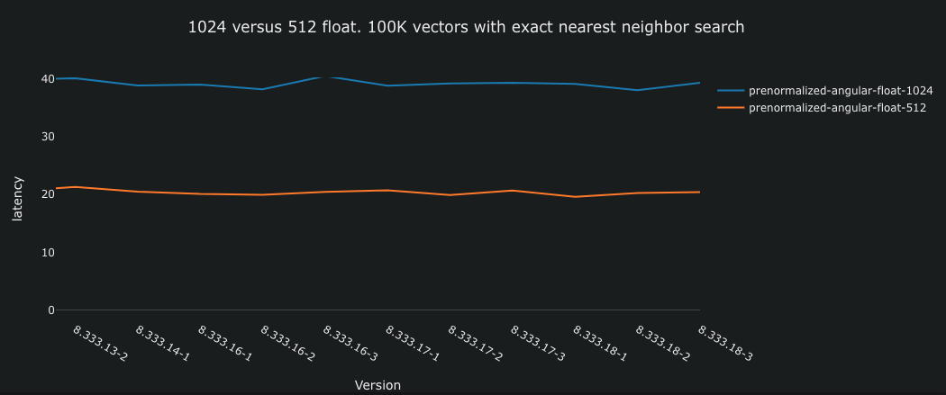
The above is from a Vespa performance
test (GitHub)
that uses the mixedbread.ai embedding model with support for MRL and
BQL and reports the end-to-end
(average) latency (ms) for exact nearest neighbor search (targetHits = 100). This test
uses the most optimized distance metric for float vectors
in Vespa, prenormalized-angular
,
which can only be used for vectors that are normalized to the same
length. The blue line represents 1024-dimensional vectors, while
the orange line represents 512-dimensional vectors. It is important
to note that this is an exact search, which performs up to 100K
comparisons. This is different from approximate searches, which are
much faster due to significantly fewer distance computations (with a degradation in accuracy).
The graph above demonstrates that reducing the float dimensions via MRL
from 1024 to 512 results in a two-fold speedup.
When converting from float vectors with cosine similarity to binary vectors, we also transition from one distance metric to another. With binary vectors, the Hamming distance becomes the appropriate measure. The Hamming distance can be calculated using efficient CPU popcount instructions over the result of a bitwise exclusive OR (XOR) operation between the two binary bit vectors. Compared to floating-point dot products, hamming involves fewer CPU instructions and less data to move between the CPU(s) and memory.
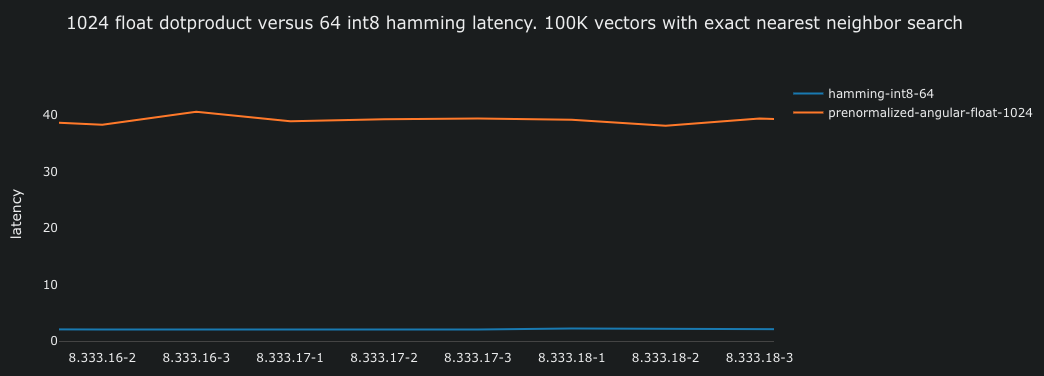
Similar to the one comparing float representations, the performance test demonstrates that calculating the hamming distance over 512-dimensional bit vectors is significantly more efficient than floating-point multiplications.
Calculating the hamming distance is approximately 20 times faster (2ms), enabling users to experience faster search and higher query throughput with the same resources. In practical terms, organizations can reduce CPU-related costs by 20x while maintaining the same query throughput as when using float embeddings.
Due to the low computing complexity and low latency search, many use cases will not need to enable HNSW indexing; an exact search might be all you need.

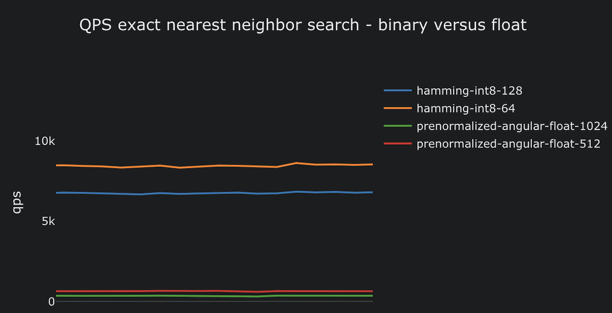
The above is part of the same test, which tests query throughput, and where the hamming metric and binary representations are much more efficient than their float counterparts. The tests run on the same hardware, embedding the same data. Approaching 10,000 queries per second with 100,000 vectors equals close to 1B hamming distance computations per second!
The huggingface-embedder functionality mentioned in the blog post makes it possible to conduct these experiments by creating multiple vector representations from the same inference call, eliminating additional inference costs (and time). The efficiency ensures that the test remains within the scope of the CI/CD pipeline at Vespa, where builds undergo performance testing (as seen on the x-axis above).
Summary
In this blog post, we have discussed the benefits of using Matryoshka Representation Learning (MRL) and Binary Quantization Learning (BQL) for embedding inference and vector indexing in Vespa. We demonstrated how to use both techniques in Vespa, with open-source models that you can embed in Vespa using the Vespa hugging-face-embedder functionality. Vespa also has first-class support for binary vectors if you want to use embedding provider APIs, see the comprehensive resources on using Cohere binary embeddings with Vespa.
The unique aspect of MRL and BQL is that they introduce minimal computational overhead during embedding model training. Both techniques are post-processing steps performed after model inference. The loss function must consider the different representations and similarities, but the additional loss function cost is insignificant compared to the model forward pass. With this negligible additional training cost, learning multiple representations instead of a single float vector representation allows for significantly cheaper and more practical retrieval implementations for online serving.
We are very excited about this direction, as it unlocks many new use cases that are no longer prohibitively expensive to serve in production—making more unstructured data useful.
The new Vespa embedder functionality for MRL and BQL is available in Vespa 8.332.5 and above; Vespa cloud tenants are already upgraded to this version.
FAQ
How does MRL/BQL compare with other retrieval and ranking strategies?
Both MRL and BQL prioritize reducing costs, even if it means sacrificing a bit on accuracy. For instance, these can be employed for initial retrieval, followed by re-ranking utilizing more advanced techniques. In the context of search, MRL and BQL serve to lower the computational and storage costs associated with the initial retrieval stage. This reduced latency (and compute) also allows pipelines to incorporate more complex models during re-ranking while adhering to overall latency SLAs (service level agreements).
Does Vespa support combining filtering with nearestNeighbors and hamming distance?
Yes, hamming distance over binary vectors represented in int8 is a
native (and mature) feature in Vespa. Hamming is exposed as a native
distance metric.
The nearest neighbor operator can be combined with filters in the
Vespa query language. See the practical guide to using Vespa nearest neighbor search.
Can Vespa combine MRL/BQL with multi-vector indexing?
Yes, it is also one of the most exciting use cases for binarized vectors. Longer texts must be chunked to fit into the embedding model capability (longer text gives a more diluted representation).
With the low cost of binary vectors, we can represent longer texts with
more chunks as vectors without significantly increasing costs. All
the new huggingface-embedder
functionality also works for array<string> inputs to represent chunks in the same
retrievable unit (document).
See Multilingual Hybrid Search with Cohere binary embeddings and Vespa for an example that uses multi-vector binary vector indexing.
Can you combine binary vectors with regular text search to implement hybrid search?
Yes, here is a concrete example using Cohere binary embeddings.
How does binary quantization relate to scalar quantization?
Both compression techniques aim to reduce storage and computation costs.
Scalar quantization (SQ) compresses float dimensions into int8 by utilizing a sample of vectors, preserving dimensionality but only achieving a compression factor of 4. It involves mapping a continuous range of float values to a set of discrete int8 values, representing 256 distinct levels. SQ requires a large set of vectors to learn the conversion for each dimension.
With a BQL-optimized embedding model, this type of analysis is included in the model training phase, as it has learned a BQ-compatible representation.
I’m confused about int8 and using it to represent binary vectors
int8 vectors can represent two distinct types:
binary vectors and vectors with the same dimensionality
as the original float representation using scalar quantization.
Notably, the latter approach utilizes the same distance metric as the float representation,
such as the angular distance. This latter approach reduces the
storage footprint by 4x, not 32x, as with BQL.
How does binary quantization relate to product quantization?
Product quantization (PQ) is used in several ANN (approximate nearest neighbor) search algorithms to compress large batches of vectors, exploiting the data distribution in these vectors. With BQL-optimized embedding models, we don’t need any post-processing of the vectors, as the model has been trained to output vectors that are compatible with Binary Quantization (BQ). In addition, BQL enables us to recreate the original lossy float representation by unpacking the bit representation, which can be used for re-scoring or as input to a DNN ranking model.
I’ve read that BQ is lossy and that the quality and accuracy is bad?
BQ is lossy because it converts a continuous range of float values into bits, and using it on vectors from an embedding model trained without the BQL objective may significantly reduce accuracy. Employing these techniques on vectors from a model that lacks training with BQL or MRL objectives would result in a more significant degradation in accuracy compared to models trained with such an objective.
I’ve read that HNSW uses a lot of memory, how does binary vectors impact HNSW?
Contrary to popular belief, the HNSW graph has a minimal impact on total memory consumption. Instead, the source vectors are the primary contributors to memory usage. Binarization offers a practical solution by reducing the storage requirements of the source vectors. It’s worth noting that both read (queries) and insert (add/update) operations necessitate graph traversal, which entails similarity calculations involving the retrieval of stored vectors.
Due to the random access pattern (to fetch source vectors) caused by HNSW graph traversal, keeping the vectors in memory is crucial for achieving meaningful insert and read performance. With binarization we both reduce the memory footprint of the vectors (32/64x) and also increase both search and indexing performance (since distance calculations are so much cheaper). In addition, there are many cases where you don’t need to build a HNSW index for retrieval, but instead use the vector representations during ranking phases. See Redefining Hybrid Search Possibilities with Vespa for a discussion on this.
How does BQ compare with the compression technique used with ColBERT?
Vespa’s ColBERT embedder (blog post) also supports binarization to reduce the storage footprint of the token-level vectors. It’s essentially the same type of compression, thresholding normalized float vectors at 0 and packing them into int8. mixedbread.ai has also trained a ColBERT checkpoint, using this in combination with their binarized single-vector model is an attractive pipeline, where retrieval phase can use the binarized single-vector representation, and ColBERT can be used to re-rank the candidates retrieved by the coarse-level hamming search.
I want to use an embedding provider instead and feed the vectors to Vespa, how can I do that?
Mixedbread.ai offers an embedding API
for getting multiple vector representations for the same inference call. This includes binary embeddings (
See the encoding_format parameter).
Cohere has embedding models and API that support obtaining multiple vector representations for the same inference API call (including binary int8 and scalar quantized int8). See our comprehensive guideon using Cohere embeddings in combination with Vespa.
I use sentence-transformers, how can I use sentence-transformers in combination with Vespa?
Sentence-transformers have great support for quantization and binarization and this is a practical example of how to use sentence-transformers in combination with Vespa.
I have more questions; I want to learn more! For those interested in learning more about Vespa or binary vectors and Vespa’s capabilities, join the Vespa community on Slack or Discord to exchange ideas, seek assistance from the community, or stay in the loop on the latest Vespa developments.