This blog post demonstrates the effectiveness of using the recently released OpenAI text-embedding-3 embeddings with Vespa.

Specifically, we are interested in the Matryoshka Representation Learning technique used in training, which lets us “shorten embeddings (i.e. remove some numbers from the end of the sequence) without the embedding losing its concept-representing properties”. This allow us to trade off a small amount of accuracy in exchange for much smaller embedding sizes, so we can store more documents and search them faster.

By using phased ranking, we can re-rank the top K results with the full embeddings in a second step. This produces accuracy on par with using the full embeddings!

We’ll use a standard information retrieval benchmark to evaluate result quality with different embedding sizes and retrieval/ranking strategies.

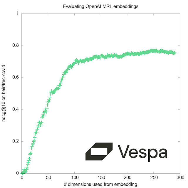
As a bonus, we’ll show at the end how we can at run-time select the number of dimensions, to evaluate how the quality improves with increasing resolution:

This blog post is also available as a runnable notebook where you can have this app up and running on Vespa Cloud in minutes ( )

Let’s get started! First, install a few dependencies:

!pip3 install -U pyvespa ir_datasets openai pytrec_eval

Examining the OpenAI embeddings

from openai import OpenAI

openai = OpenAI()

def embed(text, model="text-embedding-3-large", dimensions=3072):
   return openai.embeddings.create(input = [text], model=model, dimensions=dimensions).data[0].embedding

With these new embedding models, the API supports a dimensions parameter. Does this differ from just taking the first N dimensions?

test_input="This is just a test sentence."

full = embed(test_input)
short = embed(test_input, dimensions=8)

print(full[:8])
print(short)

[0.0035371531266719103, 0.014166134409606457, -0.017565304413437843, 0.04296272248029709,
 0.012746891938149929, -0.01731124334037304, -0.00855049304664135, 0.044189225882291794]


[0.05076185241341591, 0.20329885184764862, -0.2520805299282074, 0.6165600419044495, 
 0.18293125927448273, -0.24843446910381317, -0.1227085217833519, 0.634161651134491]

Numerically, they are not the same. But looking more closely, they differ only by a scaling factor:

scale = short[0]/full[0]
print([x * scale for x in full[:8]])
print(short)

[0.05076185241341591, 0.2032988673141365, -0.2520805173822377, 0.6165600695594861,
0.18293125124128834, -0.2484344748635628, -0.12270853156530777, 0.6341616780980419]


[0.05076185241341591, 0.20329885184764862, -0.2520805299282074, 0.6165600419044495,
 0.18293125927448273, -0.24843446910381317, -0.1227085217833519, 0.634161651134491]

It seems the shortened vector has been L2 normalized to have a magnitude of 1. By cosine similarity, they are equivalent:

from numpy.linalg import norm
from numpy import dot

def cos_sim(e1, e2):
   return dot(e1, e2)/(norm(e1)*norm(e2))

print(norm(short))

cos_sim(short, full[:8])

0.9999999899058183


0.9999999999999996

This is great, because it means that in a single API call we can get the full embeddings, and easily produce shortened embeddings just by slicing the list of numbers.

Note that text-embedding-3-large and text-embedding-3-small do not produce compatible embeddings when sliced to the same size:

cos_sim(embed(test_input, dimensions=1536), 
        embed(test_input, dimensions=1536, model="text-embedding-3-small"))

-0.03217247156447633

Getting a sample dataset

Let’s download a dataset so we have some real data to embed:

import ir_datasets
dataset = ir_datasets.load('beir/trec-covid')
print("Dataset has", dataset.docs_count(), "documents. Sample:")
dataset.docs_iter()[120]._asdict()

Dataset has 171332 documents. Sample:
{'doc_id': 'z2u5frvq',
 'text': 'The authors discuss humoral immune responses to HIV and approaches to designing vaccines that induce viral neutralizing and other potentially protective antibodies.',
 'title': 'Antibody-Based HIV-1 Vaccines: Recent Developments and Future Directions: A summary report from a Global HIV Vaccine Enterprise Working Group',
 'url': 'https://www.ncbi.nlm.nih.gov/pmc/articles/PMC2100141/',
 'pubmed_id': '18052607'}

Queries

This dataset also comes with a set of queries, and query/document relevance judgements:

print(next(dataset.queries_iter()))
print(next(dataset.qrels_iter()))

BeirCovidQuery(query_id='1', text='what is the origin of COVID-19', query='coronavirus origin', narrative="seeking range of information about the SARS-CoV-2 virus's origin, including its evolution, animal source, and first transmission into humans")
TrecQrel(query_id='1', doc_id='005b2j4b', relevance=2, iteration='0')

We’ll use these later to evaluate the result quality.

Definining the Vespa application

First, we define a Vespa schema with the fields we want to store and their type.

from vespa.package import Schema, Document, Field, FieldSet
my_schema = Schema(
            name="my_schema",
            mode="index",
            document=Document(
                fields=[
                    Field(name="doc_id", type="string", indexing=["summary"]),
                    Field(name="text", type="string", indexing=["summary", "index"], index="enable-bm25"),
                    Field(name="title", type="string", indexing=["summary", "index"], index="enable-bm25"),
                    Field(name="url", type="string", indexing=["summary", "index"]),
                    Field(name="pubmed_id", type="string", indexing=["summary", "index"]),
                    
                    Field(name="shortened", type="tensor<float>(x[256])",
                        indexing=["attribute", "index"],
                        attribute=["distance-metric: angular"]
                    ),
                    Field(name="embedding", type="tensor<float>(x[3072])",
                        indexing=["attribute"],
                        attribute=["paged", "distance-metric: angular"],
                    ),
                ],
            ),
            fieldsets=[
                FieldSet(name = "default", fields = ["title", "text"])
            ]
)

The two fields of type tensor<float>(x[3072/256]) are not in the dataset - they are tensor fields to hold the embeddings from OpenAI.

• shortened: This field holds the embedding shortened to 256 dimensions, requiring only 8.3% of the memory. index here means we will build an HNSW Approximate Nearest Neighbor index, by which we can find the closest vectors while exploring only a very small subset of the documents.

• embedding: This field contains the full size embedding. It is paged: accesses to this field may require disk access, unless it has been cached by the kernel.

We must add the schema to a Vespa application package. This consists of configuration files, schemas, models, and possibly even custom code (plugins).

from vespa.package import ApplicationPackage

vespa_app_name = "matryoshka"
vespa_application_package = ApplicationPackage(
        name=vespa_app_name,
        schema=[my_schema]
)

In the last step, we configure ranking by adding rank-profile’s to the schema.

Vespa supports has a rich set of built-in rank-features, including many text-matching features such as:

• BM25,
• nativeRank and many more.

Users can also define custom functions using ranking expressions.

The following defines three runtime selectable Vespa ranking profiles:

• exact uses the full-size embedding
• shortened uses only 256 dimensions (exact, or using the approximate nearest neighbor HNSW index)
• rerank uses the 256-dimension shortened embeddings (exact or ANN) in a first phase, and the full 3072-dimension embeddings in a second phase. By default the second phase is applied to the top 100 documents from the first phase.

This idea of re-ranking the top hits is well-supported in Vespa and already suggested by the researchers who developed MRL:

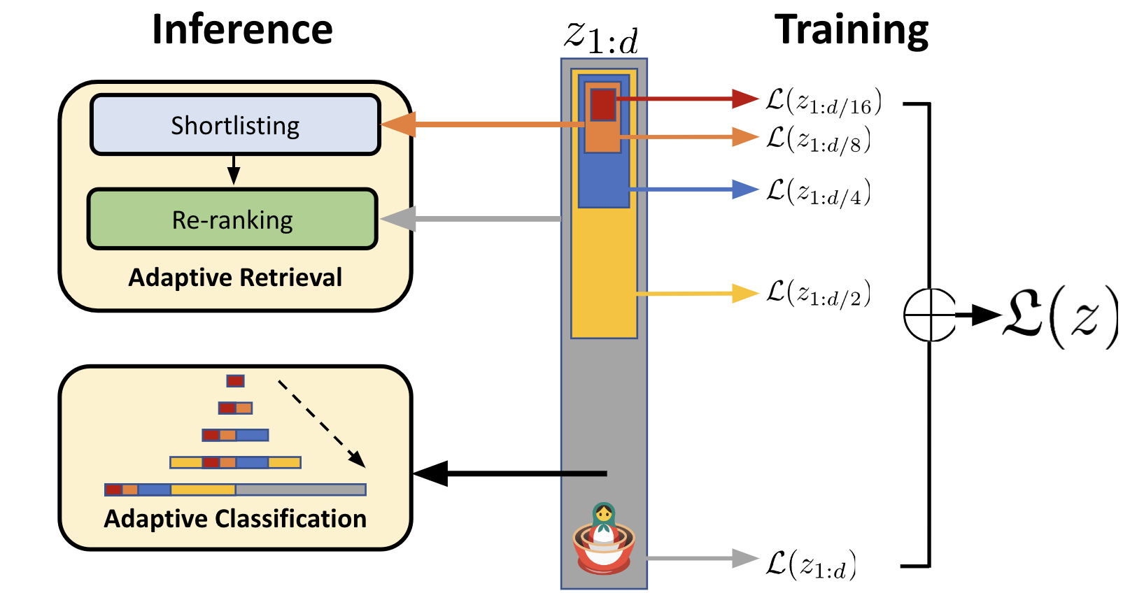
Illustration from their excellent blog post. Now let’s see what the corresponding rank profiles look like:

from vespa.package import RankProfile, Function, FirstPhaseRanking, SecondPhaseRanking

exact = RankProfile(
    name="exact",
    inputs=[
        ("query(q3072)", "tensor<float>(x[3072])")
        ],
    functions=[
        Function(
            name="cos_sim",
            expression="closeness(field, embedding)"
        )
    ],
    first_phase=FirstPhaseRanking(
        expression="cos_sim"
    ),
    match_features=["cos_sim"]
)
my_schema.add_rank_profile(exact)


shortened = RankProfile(
    name="shortened",
    inputs=[
        ("query(q256)", "tensor<float>(x[256])")
        ],
    functions=[
        Function(
            name="cos_sim_256",
            expression="closeness(field, shortened)"
        )
    ],
    first_phase=FirstPhaseRanking(
        expression="cos_sim_256"
    ),
    match_features=["cos_sim_256"]
)
my_schema.add_rank_profile(shortened)


rerank = RankProfile(
    name="rerank",
    inputs=[
        ("query(q3072)", "tensor<float>(x[3072])"),
        ("query(q256)", "tensor<float>(x[256])")
        ],
    functions=[
        Function(
            name="cos_sim_256",
            expression="closeness(field, shortened)"
        ),
        Function(
            name="cos_sim_3072",
            expression="cosine_similarity(query(q3072), attribute(embedding), x)"
        ),
    ],
    first_phase=FirstPhaseRanking(
        expression="cos_sim_256"
    ),
    second_phase=SecondPhaseRanking(
        expression="cos_sim_3072"
    ),
    match_features=["cos_sim_256", "cos_sim_3072"]
)
my_schema.add_rank_profile(rerank)

For an example of a hybrid rank-profile which combines semantic search with traditional text retrieval such as BM25, see the previous blog post: Turbocharge RAG with LangChain and Vespa Streaming Mode for Sharded Data

Deploy the application to Vespa Cloud

With the configured application, we can deploy it to Vespa Cloud. It is also possible to deploy the app using docker; see the Hybrid Search - Quickstart guide for an example of deploying a Vespa app using the vespaengine/vespa container image.

See the full notebook for complete details on onboarding Vespa Cloud and deployment details.

Get OpenAI embeddings for documents in the dataset

When producing the embeddings, we concatenate the title and text into a single string. We could also have created two separate embedding fields for text and title, combining the rank scores for these fields in a Vespa rank expression.

import concurrent.futures

def embed_doc(doc):
  embedding = embed((doc.title + " " + doc.text)[:8192]) # we crop the ~25 documents which are longer than the context window
  shortened = embedding[0:256]
  return {
      "doc_id": doc.doc_id,
      "text": doc.text,
      "title": doc.title,
      "url": doc.url,
      "pubmed_id": doc.pubmed_id,
      
      "shortened": {"type":"tensor<float>(x[256])","values":shortened},
      "embedding": {"type":"tensor<float>(x[3072])","values":embedding}
  }

with concurrent.futures.ThreadPoolExecutor(max_workers=10) as executor:
        my_docs_to_feed = list(executor.map(embed_doc, dataset.docs_iter()[:100])) # only embed 100 docs while developing

Feeding the dataset and embeddings into Vespa

Now that we have parsed the dataset and created an object with the fields that we want to add to Vespa, we must format the object into the format that PyVespa accepts. Notice the fields, id and groupname keys. The groupname is the key that is used to shard and co-locate the data and is only relevant when using Vespa with streaming mode.

from typing import Iterable
def vespa_feed(user:str) -> Iterable[dict]:
    for doc in reversed(my_docs_to_feed):
        yield {
            "fields": doc,
            "id": doc["doc_id"],
            "groupname": user
        }

Now, we can feed to the Vespa instance (app), using the feed_iterable API, using the generator function above as input with a custom callback function.

from vespa.io import VespaResponse

def callback(response:VespaResponse, id:str):
    if not response.is_successful():
        print(f"Document {id} failed to feed with status code {response.status_code}, url={response.url} response={response.json}")

app.feed_iterable(schema="my_schema", iter=vespa_feed(""), callback=callback, max_queue_size=8000, max_workers=64, max_connections=128)

Embedding the queries

We need to obtain embeddings for the queries from OpenAI. If only using the shortened embedding for the query, you should specify this in the OpenAI API call to reduce latency.

queries = []
for q in dataset.queries_iter():
    queries.append({'text': q.text, 'embedding': embed(q.text), 'id': q.query_id})

Querying data

Now we can query our data. We’ll do it in a few different ways, using the rank profiles we defined in the schema:

• Exhaustive (exact) nearest neighbor search with the full embeddings (3072 dimensions)
• Exhaustive (exact) nearest neighbor search with the shortened 256 dimensions
• Approximate nearest neighbor search, using the 256 dimension ANN HNSW index
• Approximate nearest neighbor search, using the 256 dimension ANN HNSW index in the first phase, then reranking top 100 hits with the full embeddings

The query request uses the Vespa Query API and the Vespa.query() function supports passing any of the Vespa query API parameters.

Read more about querying Vespa in:

• Vespa Query API
• Vespa Query API reference
• Vespa Query Language API (YQL)

import json

def query_exact(q):
    return session.query(
        yql="select doc_id, title from my_schema where ({targetHits: 10, approximate:false}nearestNeighbor(embedding,q3072)) limit 10",
        ranking="exact",
        timeout=10,
        body={            
            "presentation.timing": "true",
            "input.query(q3072)": q['embedding']            
        }
    )

def query_256(q):
    return session.query(
        yql="select doc_id from my_schema where ({targetHits: 10, approximate:false}nearestNeighbor(shortened,q256)) limit 10",
        ranking="shortened",
        timeout=10,
        body={            
            "presentation.timing": "true",
            "input.query(q256)": q['embedding'][:256]
        }
    )

def query_256_ann(q):
    return session.query(
        yql="select doc_id from my_schema where ({targetHits: 100, approximate:true}nearestNeighbor(shortened,q256)) limit 10",
        ranking="shortened",
        timeout=10,
        body={            
            "presentation.timing": "true",
            "input.query(q256)": q['embedding'][:256]
        }
    )

def query_rerank(q):
    return session.query(
        yql="select doc_id from my_schema where ({targetHits: 100, approximate:true}nearestNeighbor(shortened,q256)) limit 10",
        ranking="rerank",
        timeout=10,
        body={            
            "presentation.timing": "true",
            "input.query(q256)": q['embedding'][:256],
            "input.query(q3072)": q['embedding']
        }
    )

print("Sample query:", queries[0]['text'])
with app.syncio() as session:
    print(json.dumps(query_rerank(queries[0]).hits[0], indent=2))

Sample query: what is the origin of COVID-19


{
  "id": "index:matryoshka_content/0/16c7e8749fb82d3b5e37bedb",
  "relevance": 0.6591723960884718,
  "source": "matryoshka_content",
  "fields": {
    "matchfeatures": {
      "cos_sim_256": 0.5481410972571522,
      "cos_sim_3072": 0.6591723960884718
    },
    "doc_id": "beguhous"
  }
}

Here’s the top result from the first query. Notice the matchfeatures that returns the match-features from the rank-profile.

Now for each method of querying, we’ll run all our queries and note the rank of each document in the response:

global qt

def run_queries(query_function):
    print("\nrun", query_function.__name__, )
    results = {}
    for q in queries:
        response = query_function(q)
        assert(response.is_successful())        
        print(".", end="")
        results[q['id']] = {}
        for pos, hit in enumerate(response.hits, start=1):
            global qt 
            qt += float(response.get_json()['timing']['querytime'])
            results[q['id']][hit['fields']['doc_id']] = pos
    return results

query_functions = ( query_exact, query_256, query_256_ann, query_rerank )
runs = {}

with app.syncio() as session:
    for f in query_functions:
        qt=0
        runs[f.__name__] = run_queries(f)
        print(" avg query time {:.4f} s".format(qt/len(queries)))

run query_exact
.................................................. avg query time 2.7918 s

run query_256
.................................................. avg query time 0.3040 s

run query_256_ann
.................................................. avg query time 0.0252 s

run query_rerank
.................................................. avg query time 0.0310 s

The query time numbers here are NOT a proper benchmark but can illustrate some significant trends for this case:

• Doing exact NN with 3072 dimensions is too slow and expensive for many use cases
• Reducing dimensionality to 256 reduces latency by an order of magnitude
• Using an ANN index improves query time by another order of magnitude
• Re-ranking the top 100 results with the full embedding causes only a slight increase

We could use more cores per search or sharding over multiple nodes to improve latency and handle larger content volumes.

Evaluating the query results

We need to get the query relevance judgements into the format supported by pytrec_eval:

qrels = {}

for q in dataset.queries_iter():
    qrels[q.query_id] = {}

for qrel in dataset.qrels_iter():
    qrels[qrel.query_id][qrel.doc_id] = qrel.relevance

With that done, we can check the scores for the first query:

for docid in runs['query_256_ann']['1']:
    score = qrels['1'].get(docid)
    print(docid, score or "-")

beguhous 2
k9lcpjyo 2
pl48ev5o 2
jwxt4ygt 2
dv9m19yk 1
ft4rbcxf 1
h8ahn8fw 2
6y1gwszn 2
3xusxrij -
2tyt8255 1

A lot of ‘2’, that is, ‘highly relevant’ results: Looks promising! Now we can use trec_eval to evaluate all the data for each run. The quality measure we use here is nDCG@10 - Normalized Discounted Cumulative Gain, computed for the first 10 results of each query. The evaluations are per-query so we compute and report the average per run.

import pytrec_eval

def evaluate(run):
    evaluator = pytrec_eval.RelevanceEvaluator(
        qrels, {'ndcg_cut.10'})
    evaluation = evaluator.evaluate(run)
    
    sum = 0
    for ev in evaluation:
        sum+=evaluation[ev]['ndcg_cut_10']
    return sum/len(evaluation)

for run in runs:
  print(run, "\tndcg_cut_10: {:.4f}".format(evaluate(runs[run])))

query_exact 	ndcg_cut_10: 0.7870
query_256 	ndcg_cut_10: 0.7574
query_256_ann 	ndcg_cut_10: 0.7552
query_rerank 	ndcg_cut_10: 0.7886

Conclusions

What do the numbers mean? They are good, highly relevant results. This is no great surprise, as the OpenAI embedding models are reported to score high on the Massive Text Embedding Benchmark, of which our BEIR/TREC-COVID dataset is a part.

More interesting to us, querying with the first 256 dimensions still gives quite good results, while requiring only 8.3% of the memory. We also note that although the HNSW index is an approximation, result quality is impacted very little, while producing the results an order of magnitude faster.

When adding a second phase to re-rank the top 100 hits using the full embeddings, the results are as good as the exact search, while retaining the lower latency, giving us the best of both worlds.

Bonus content: Selecting the number of dimensions

The choice of the embedding sizes (256 and 3072) in this experiment was fairly arbitrary. While they gave good results, we were curious: How low could we go? Is it beneficial to stay within the set of dimensions for which the model was trained?

Re-embedding the content with a large number of different values for the “dimensions” parameter would be costly and time-consuming. And even if we did this (or sliced the embeddings to produce smaller embeddings ourselves), deploying a new Vespa application and importing the results into it for each value to test would be very slow.

Fortunately the Vespa rank expression language supports slicing!

Vespa rank expressions are highly optimized and compiled to native code by LLVM at deploy time. Optimization is harder if the sizes of types are not know in this step, thus we can’t currently write a single rank profile where the number of dimensions is a parameter - but by creating one rank profile per value we’d like to test, we can select it - per query - at execution time. These we can produce with a simple template:

    for i in range(1, 3072+1):
        dims = RankProfile(
            name="dims_"+str(i),
            inputs=[
                ("query(q"+str(i)+")", "tensor<float>(x["+str(i)+"])"),
                ],
            functions=[
                Function(
                    name="cos_sim_"+str(i),
                    expression="cosine_similarity(" + 
                        "tensor<float>(x["+str(i)+"])(attribute(embedding){x:(x)}), " + 
                        "tensor<float>(x["+str(i)+"])(query(q"+str(i)+"){x:(x)})"+
                    ", x)"
                ),
            ],
            first_phase=FirstPhaseRanking(
                expression="cos_sim_"+str(i)
            ),
            match_features=["cos_sim_"+str(i)]
        )
        my_schema.add_rank_profile(dims)

By re-deploying with this new schema and performing some trivial modifications to the query code above, you can efficiently test different values to find the right performance/accuracy trade-off. Our graph corroborates the claim by the authors of the MRL paper; while training uses a fixed set of ‘doll sizes’, there are no ‘magic numbers’ that give better results with the resulting model.

For those interested in learning more about Vespa, join the Vespa community on Slack or Discord to exchange ideas, seek assistance from the community, or stay in the loop on the latest Vespa developments.